Day 08
Thursday, Feb 23, 2017
Ch 2 Method of separation of variables, cont'd
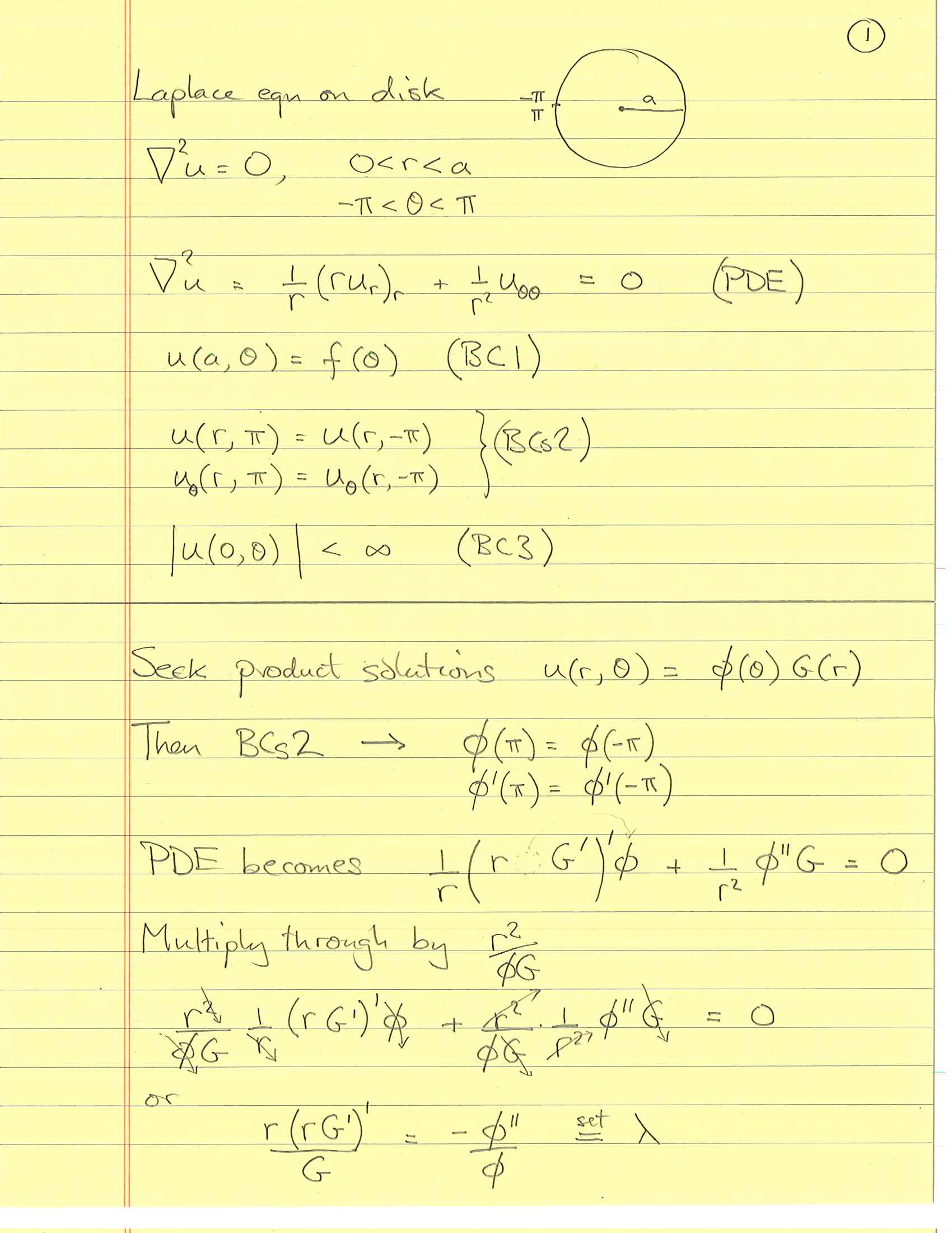
2.5 Laplace's equation in 2D, cont'd
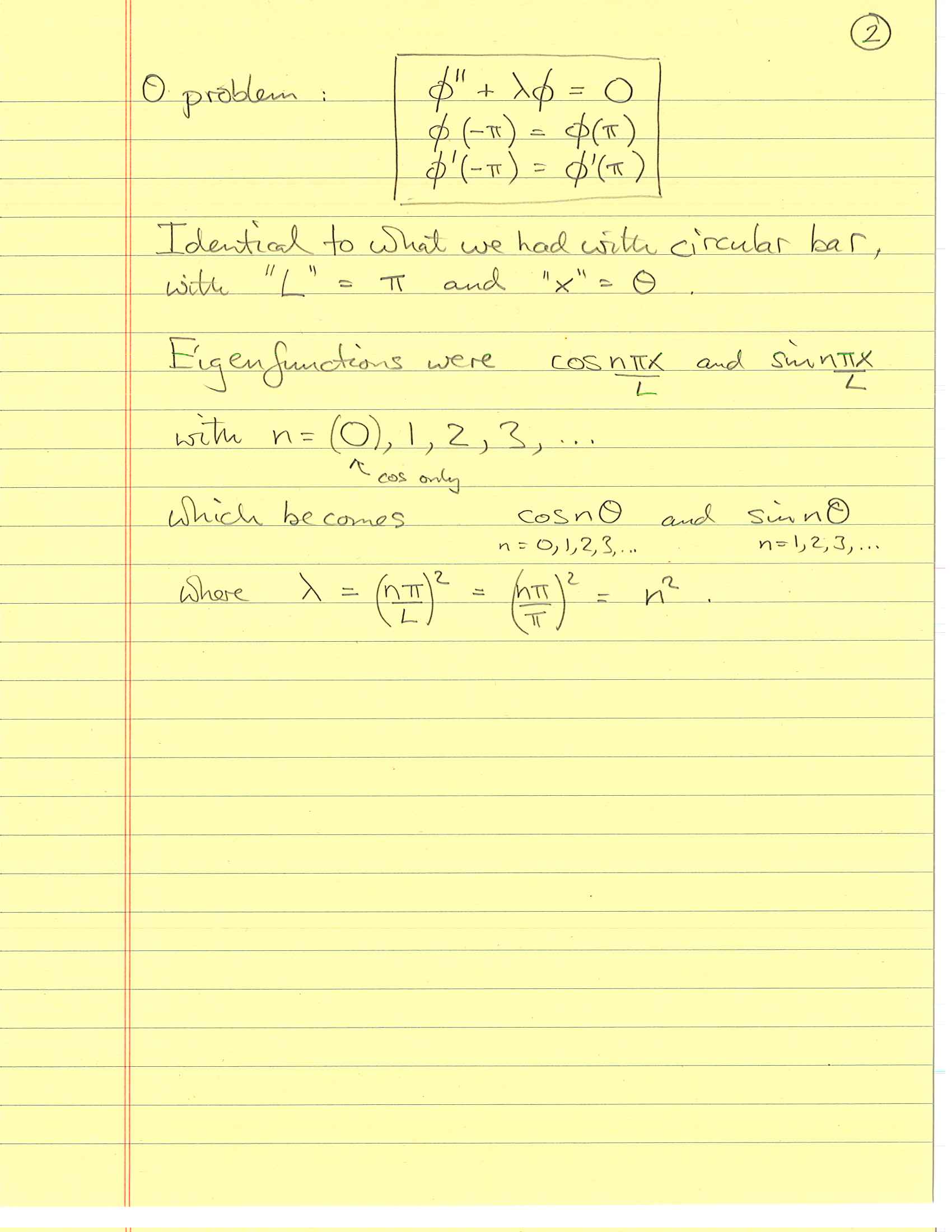
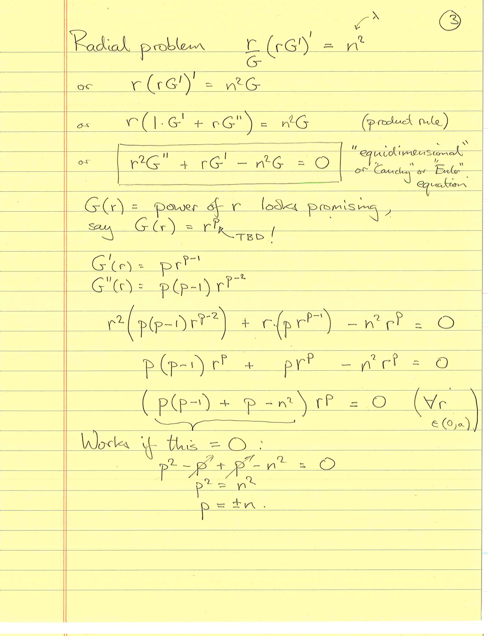
2.5.2 Disk
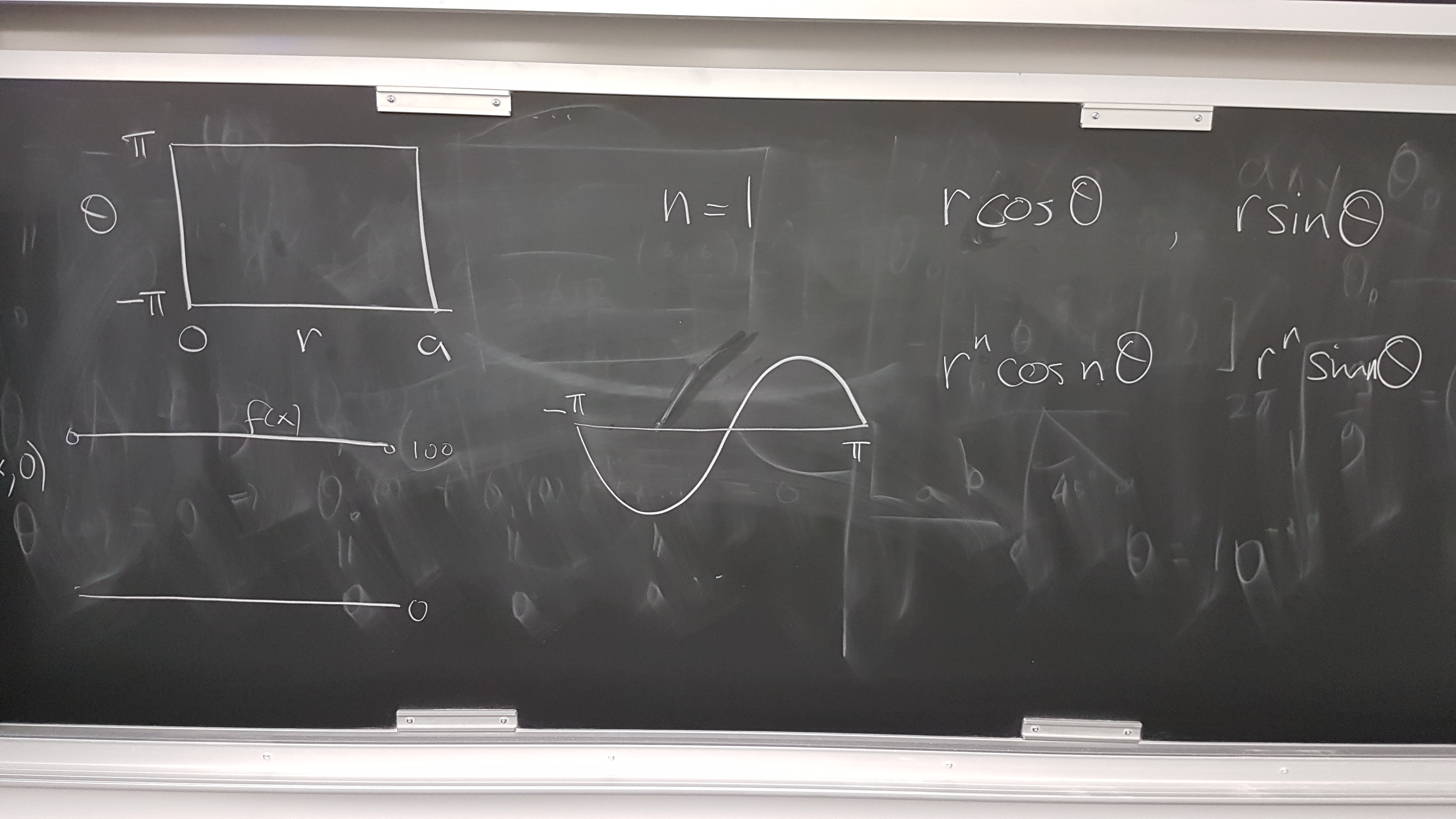
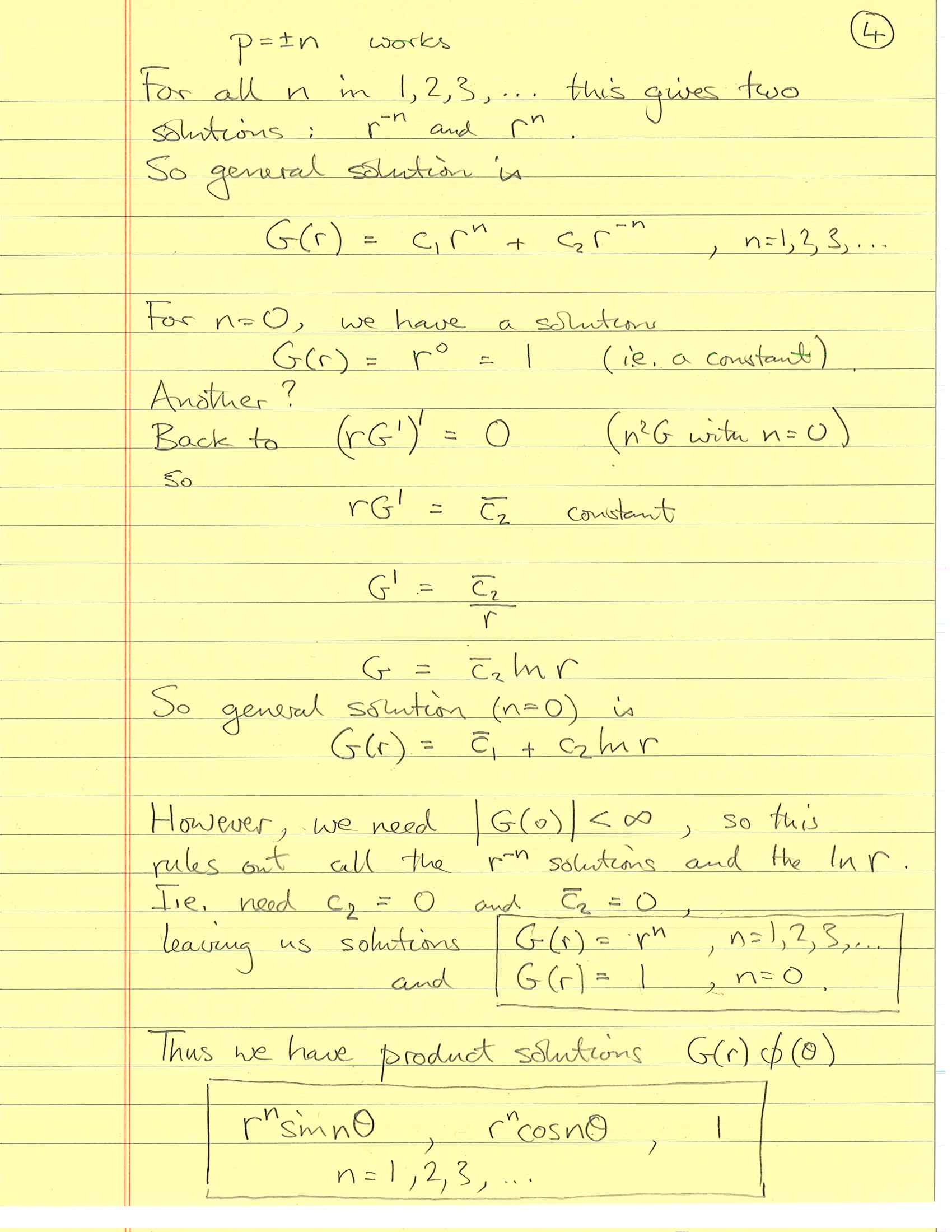
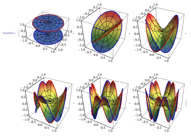
Let's look at some these product solutions:
Another way of visualizing them:
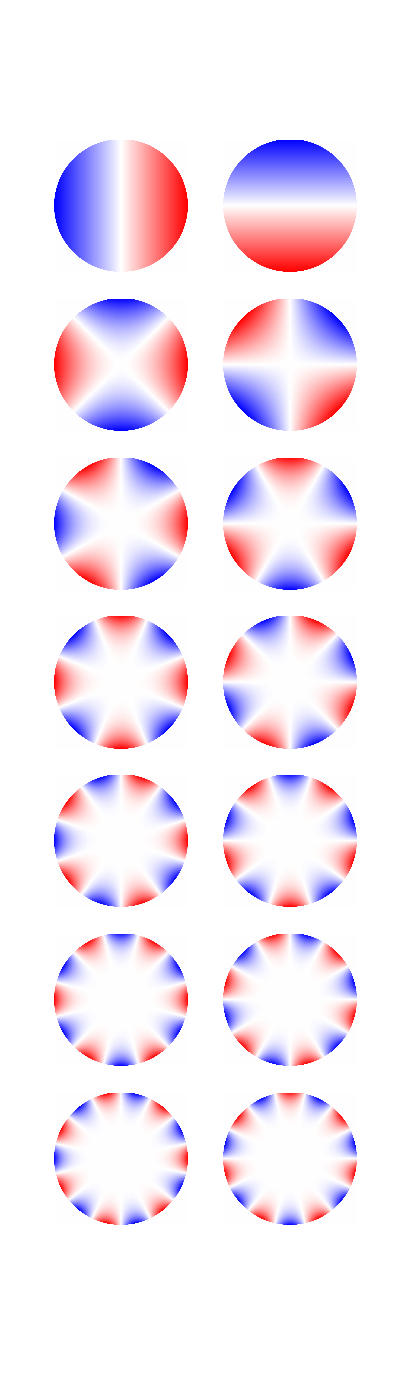
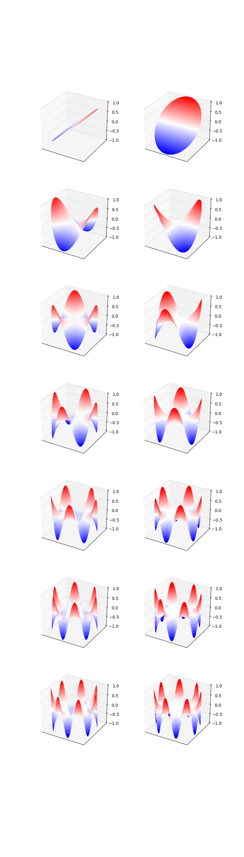
from numpy import *
%matplotlib inline
import matplotlib.pyplot as pl

M = 7
x = linspace(-1,1,500)
y = linspace(-1,1,500)
X,Y = meshgrid(x,y)
R = sqrt(X*X+Y*Y)
Theta = arctan2(Y,X)

pl.figure(figsize=(4,2*M))
for nm1 in range(M):
         n = nm1+1
         pl.subplot(M,2,2*n-1)
         Z = R**n*cos(n*Theta) # evaluation of the function on the grid
         Z[R>1]=0
         im = pl.imshow(Z,cmap=pl.cm.bwr) # drawing the function
         pl.xticks([]); pl.yticks([])

         pl.subplot(M,2,2*n-1+1)
         Z = R**n*sin(n*Theta) # evaluation of the function on the grid
         Z[R>1]=0
         im = pl.imshow(Z,cmap=pl.cm.bwr) # drawing the function
         pl.xticks([]); pl.yticks([])
pl.savefig('disk_eigenfunctions.png')
from mpl_toolkits.mplot3d import Axes3D

M = 7
r = linspace(0,1,30)
theta = linspace(0,2*pi,250)
R,Theta = meshgrid(r,theta)

X = R*cos(Theta)
Y = R*sin(Theta)

fig = pl.figure(figsize=(8,4*M))
for nm1 in range(M):
         n = nm1+1
         Z = R**n*cos(n*Theta) # evaluation of the function on the grid
         #Z[R>1]=0
         ax = fig.add_subplot(M,2,2*n-1, projection='3d')
         ax.plot_surface(X, Y, Z, cmap=pl.cm.cool,linewidth=0, antialiased=True)
         pl.xticks([]); pl.yticks([])

         pl.subplot(M,2,2*n-1+1)
         Z = R**n*sin(n*Theta) # evaluation of the function on the grid
         #Z[R>1]=0
         ax = fig.add_subplot(M,2,2*n-1+1, projection='3d')
         ax.plot_surface(X, Y, Z, cmap=pl.cm.cool,linewidth=0, antialiased=True)
         pl.xticks([]); pl.yticks([])
pl.savefig('disk_eigenfunctions_3d.png')
# Why so few facets??
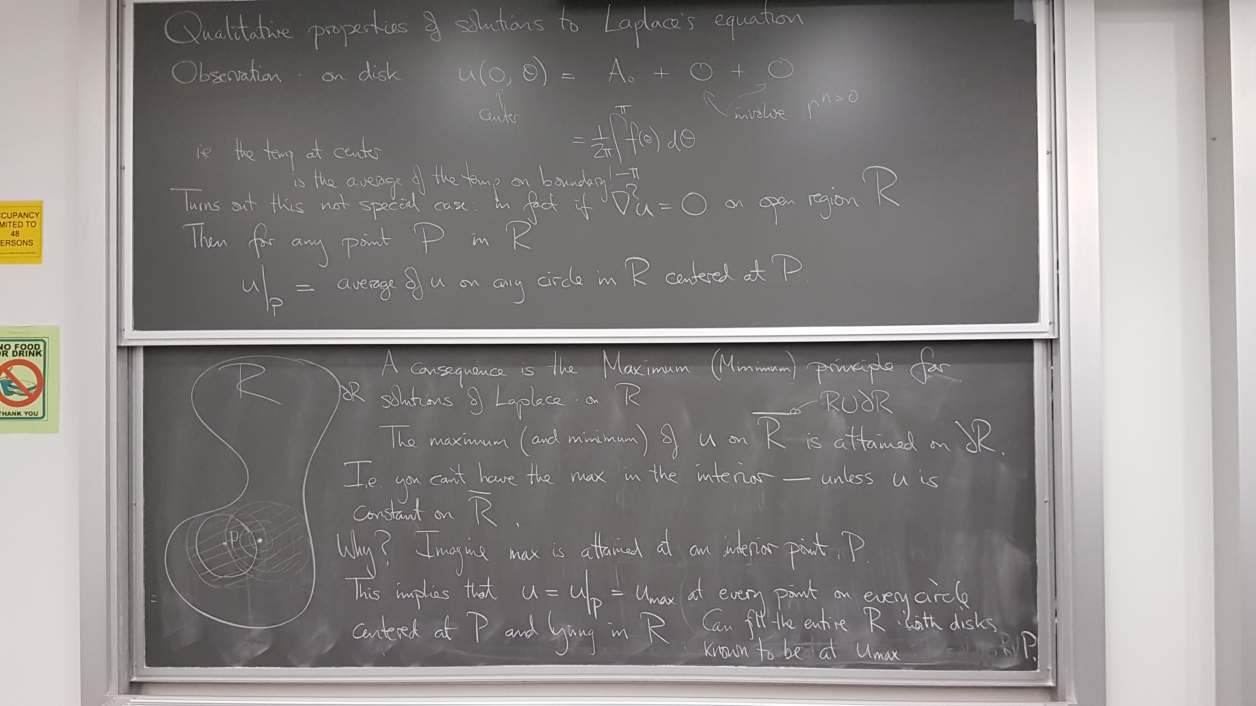
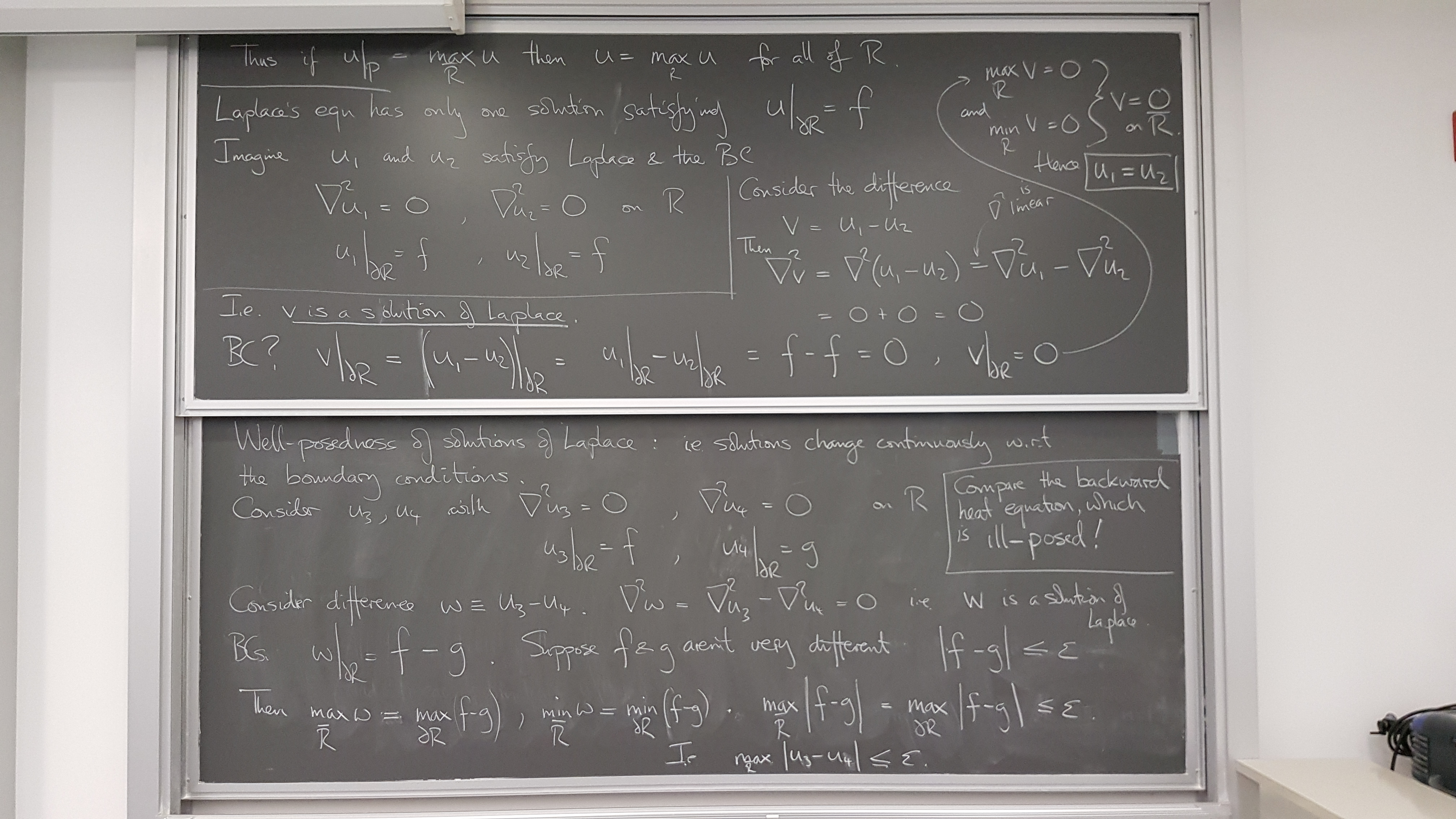
2.5.4 Qualitative properties
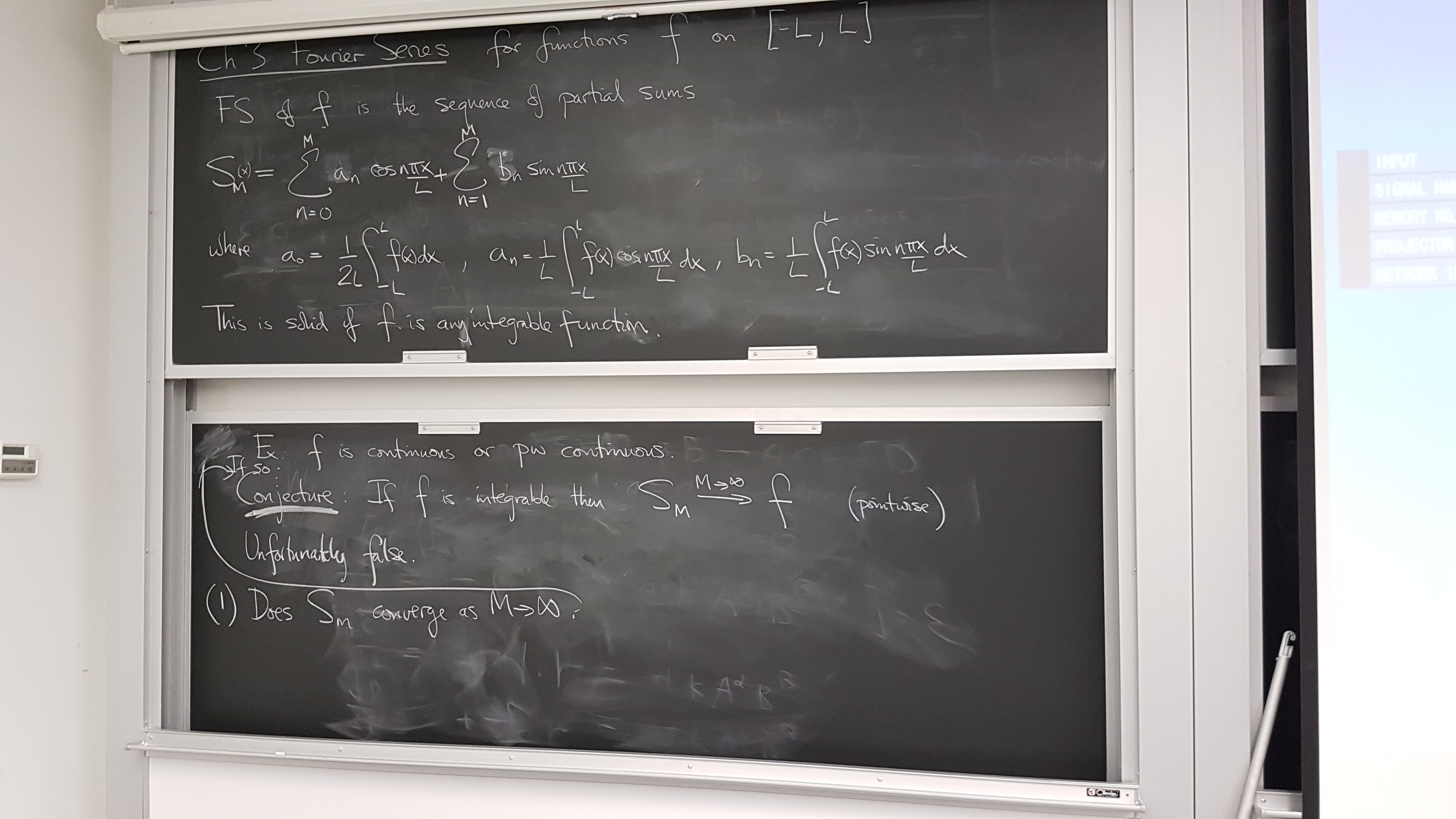
Ch 3 Fourier Series
Definition
Periodic extension of f on [-L,L).
Convergence? Let's explore a little ...