Day 14
Tuesday, March 28, 2017
Ch 5: Sturm-Liouville problems, cont'd
Let's generalize the problems we've been looking at so far.
Heat flow in a bar of non-uniform cross-section
Going way back to Ch. 1, we have the following PDE for the temperature profile u(x, t) in a slender bar, allowing all the material properties all to be non-constant:
c(x)ρ(x)A(x)ut(x, t) = (A(x)K0(x)ux(x, t))x.
Setting u(x, t) = φ(x)h(t) this says
c(x)ρ(x)A(x)φ(x)h′(t) = (A(x)K0(x)φ′(x))′h(t)
which separates as
(h′(t))/(h(t)) = ((A(x)K0(x)φ′(x))′)/(c(x)ρ(x)A(x)φ(x)) = − λ
giving
h′(t) = − λh(t),
(A(x)K0(x)φ′(x))′ + λc(x)ρ(x)A(x)φ(x) = 0.
Let us assume the bar has uniform material composition, so that K0 ρ and c do not depend on location - say K0(x) = 1, ρ(x) = 1, c(x) = 1, but we allow the cross-sectional area, A(x), to vary.
Also, let's assume we will hold the left-hand end (x=0) at 0 degrees, and insulate the opposite end (x=L) so the flux is zero at x=L.
Then the spatial eigenproblem becomes:
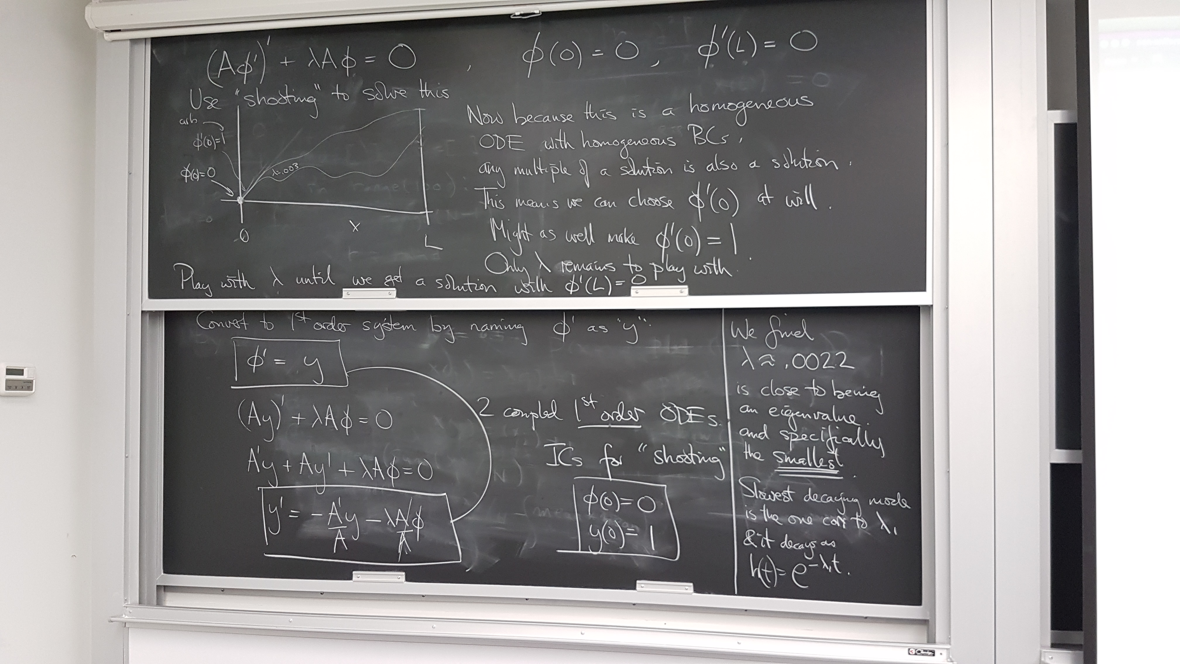
(A(x)φ′(x))′ + λA(x)φ(x) = 0,
φ(0) = 0, φ′(L) = 0.
If we can find some solutions of this ODE BVP, then they are spatial eigenfunctions of the PDE. A priori they might not be orthogonal, though, and it might be possible that we'll have only a limited number of them. (The Sturm-Liouville theory will answer these worries.)
Let us pick some specific varying cross-section function, A(x) and then use an ODE solver in Python to try and find the eigenvalues and eigenfunctions for the corresponding ODE for φ(x) using the "shooting" method I will describe.
Exercise 1
Suppose we choose A(x) = 1.1 + cos(2πx)/(L)

(Python code to draw bar here)
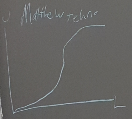
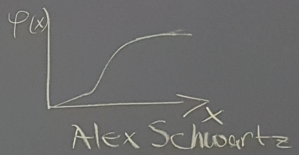
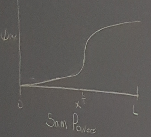
What do you think the slowest-decaying (i.e. smallest λ) eigenfunction will look like in this problem? Think about it, then draw your guess on the board, and sign it!
Exercise 2
Will the λ1 for this non-uniform bar be larger (i.e. mode decays faster) or smaller (i.e. mode decays slower) than the λ1 for the uniform bar?
Numerically compute the first eigenfunction and the corresponding eigenvalue
Numerical ODE solvers are all set up to solve systems of 1st order ODES. So we'll need to convert our 2nd order ODE to that form.
First expand the first term of the ODE using the product rule as:
(Aφ′)′ = Aφ′′ + A′φ′.
Then continue by defining φ′ = ψ, say.
GOT TO HERE Day 13.
Specifically, let us find the first (smallest) several eigenvalues and make a plot the corresponding eigenfunctions.
Shooting to find eigenvalues and eigenfunctions
Smallest eigenvalue
Our first shots:
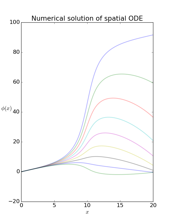
ringland@blue:~/public_html/418$ py non-uniform_bar.py
lambda = 0.0                 : phi'(L) = 1.000000444587765
lambda = 0.01                : phi'(L) = -2.5218656367781027
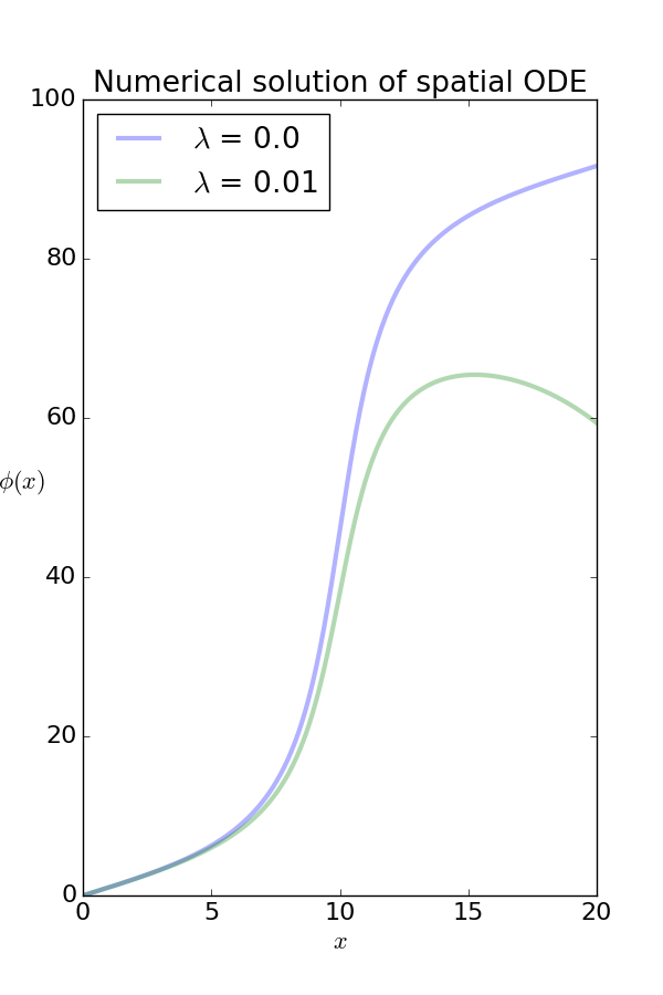
We seem to have captured the smallest eigenvalue somewhere between 0 and 0.01. Let's look closer ...
ringland@blue:~/public_html/418$ py non-uniform_bar.py
lambda = 0.0                 : phi'(L) = 1.000000444587765
lambda = 0.00025             : phi'(L) = 0.8808779967983755
lambda = 0.0005              : phi'(L) = 0.7635397347055736
lambda = 0.00075             : phi'(L) = 0.6479696072306252
lambda = 0.001               : phi'(L) = 0.5341519836659785
lambda = 0.00125             : phi'(L) = 0.42207088354630423
lambda = 0.0015              : phi'(L) = 0.31171066959066557
lambda = 0.00175             : phi'(L) = 0.20305583065389565
lambda = 0.002               : phi'(L) = 0.09609071981800561
lambda = 0.00225             : phi'(L) = -0.0091995598926174
lambda = 0.0025              : phi'(L) = -0.1128306966423111
lambda = 0.00275             : phi'(L) = -0.21481770101420766
[remainder omitted]
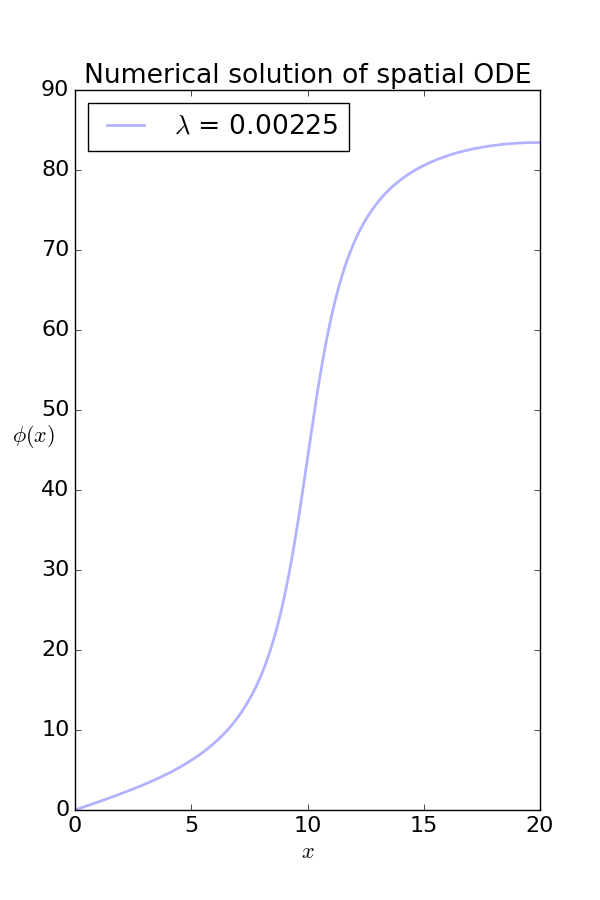
So our smallest eigenvalue looks to be λ1 ≈ 0.00225. Therefore this is the picture to compare your prediction sketch of Day 13:
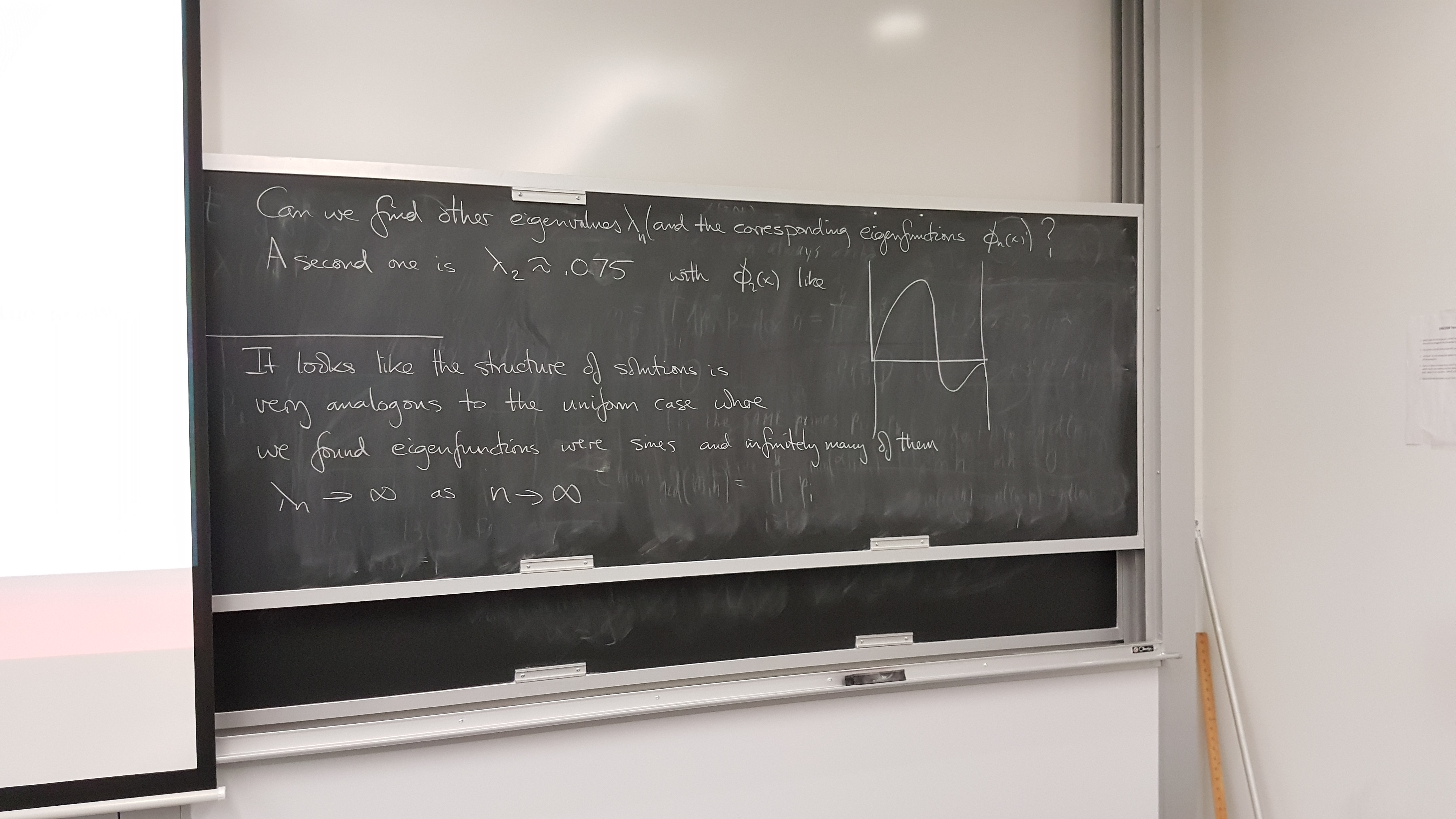
How about a second eigenvalue?
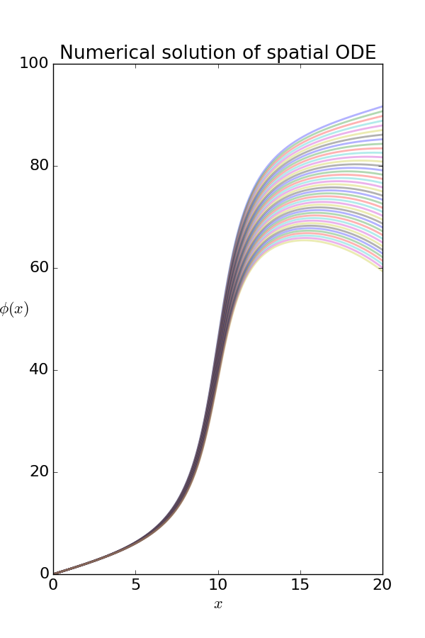
We'll try going up to lambda = 0.08:
ringland@blue:~/public_html/418$ py non-uniform_bar.py
lambda = 0.0                 : phi'(L) = 1.000000444587765
lambda = 0.01                : phi'(L) = -2.5218656367781027
lambda = 0.02                : phi'(L) = -4.051481202064394
lambda = 0.03                : phi'(L) = -4.279579716989934
lambda = 0.04                : phi'(L) = -3.7201642805170243
lambda = 0.05                : phi'(L) = -2.746567965301901
lambda = 0.06                : phi'(L) = -1.6213808523489763
lambda = 0.07                : phi'(L) = -0.521142817358817
lambda = 0.08                : phi'(L) = 0.44341238297076263
Good! We have passed through zero-slope at x=L again. Zooming in a bit ...
ringland@blue:~/public_html/418$ py non-uniform_bar.py
lambda = 0.07                : phi'(L) = -0.521142817358817
lambda = 0.07200000000000001 : phi'(L) = -0.31479480787128866
lambda = 0.07400000000000001 : phi'(L) = -0.11465232772346716
lambda = 0.076               : phi'(L) = 0.07873781172935942
lambda = 0.078               : phi'(L) = 0.2648969971065854
lambda = 0.08                : phi'(L) = 0.44341238297076263
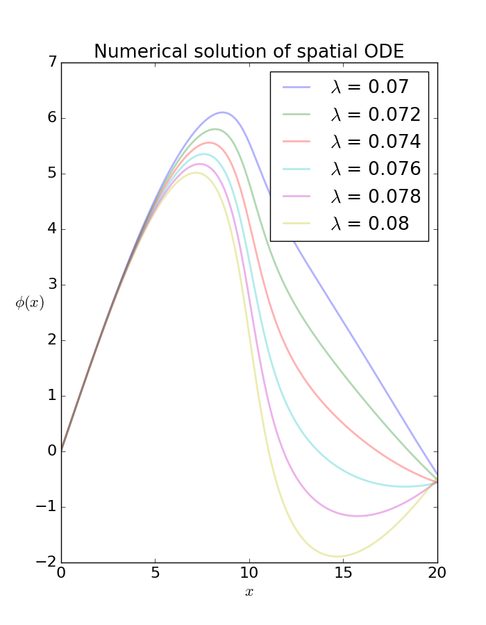
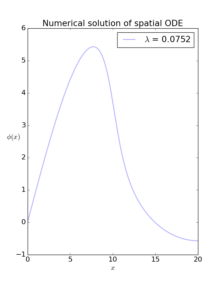
Looks like λ2 ≈ 0.0752:
We can continue to increase lambda to find additional eigenvalues. Here 50 values between 0.0753 and 1:
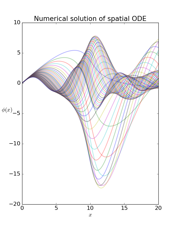
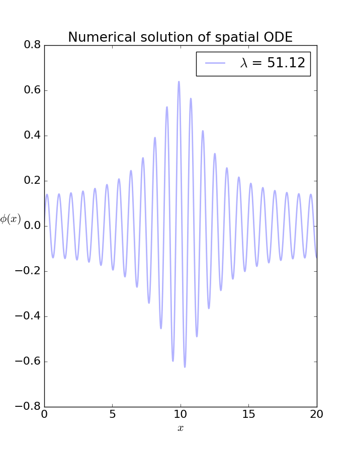
Looks like we passed over several eigenvalues in that range. And we can go higher still. The next set of shots shows there is an eigenvalue λ ≈ 51.12:
ringland@blue:~/public_html/418$ py non-uniform_bar.py
lambda = 51.0                : phi'(L) = -0.16168482969249998
lambda = 51.02               : phi'(L) = -0.1339811444223814
lambda = 51.04               : phi'(L) = -0.10617754016583797
lambda = 51.06               : phi'(L) = -0.078296680951926
lambda = 51.08               : phi'(L) = -0.05035974923012558
lambda = 51.1                : phi'(L) = -0.022388623013249467
lambda = 51.12               : phi'(L) = 0.00559413827806367
lambda = 51.14               : phi'(L) = 0.033568092967984964
lambda = 51.16               : phi'(L) = 0.06150911907898296
lambda = 51.18               : phi'(L) = 0.08939673734343624
lambda = 51.2                : phi'(L) = 0.11720962485962341
It would be nice to compare and contrast with the eigenthings for a uniform bar, and see if our eigenvalues and eigenfunctions (especially λ1 and φ1(x)) for this particular non-uniform bar "make sense".
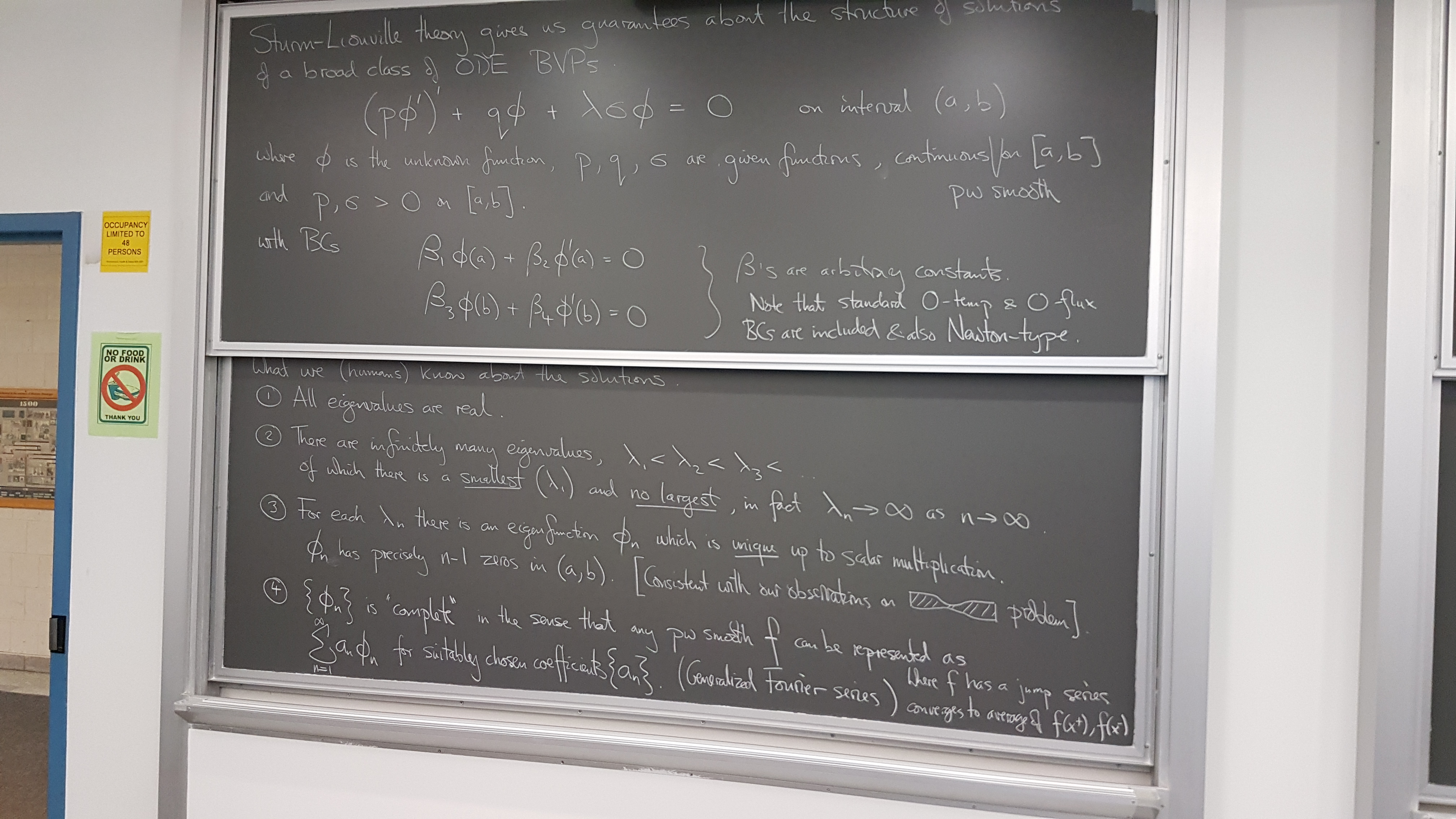
Things we can say about all Sturm-Liouville problems
5 very definitive things
Proofs of three of the things
Eigenvalues are all real
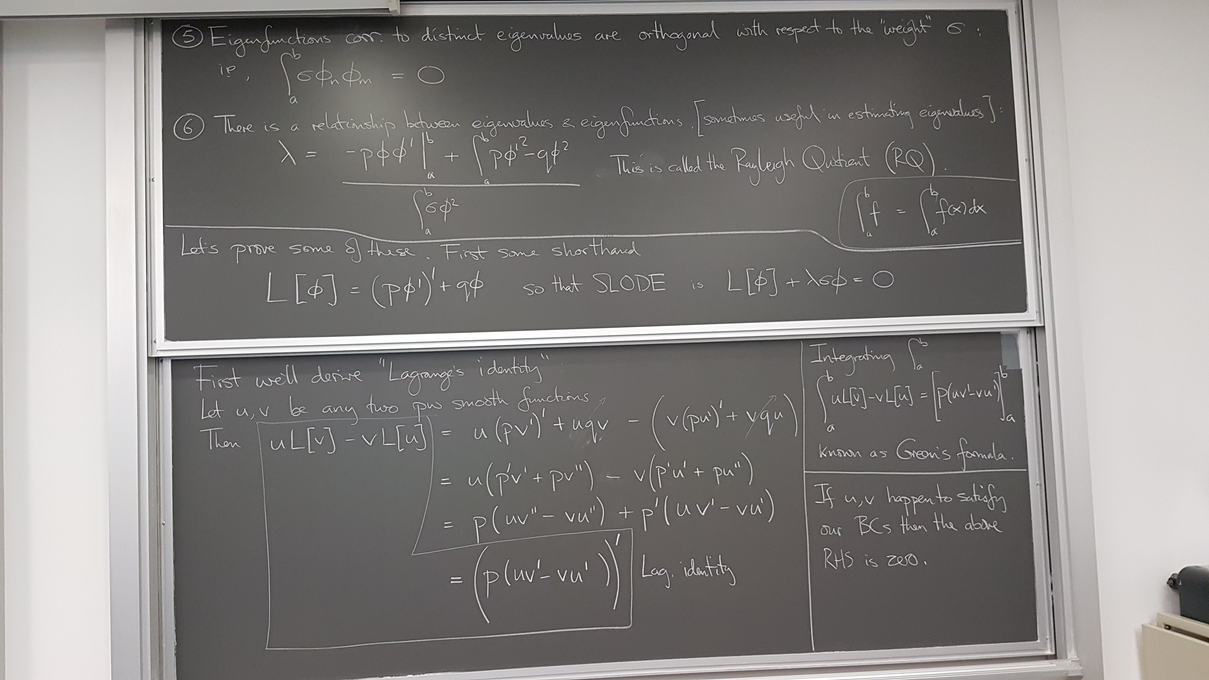
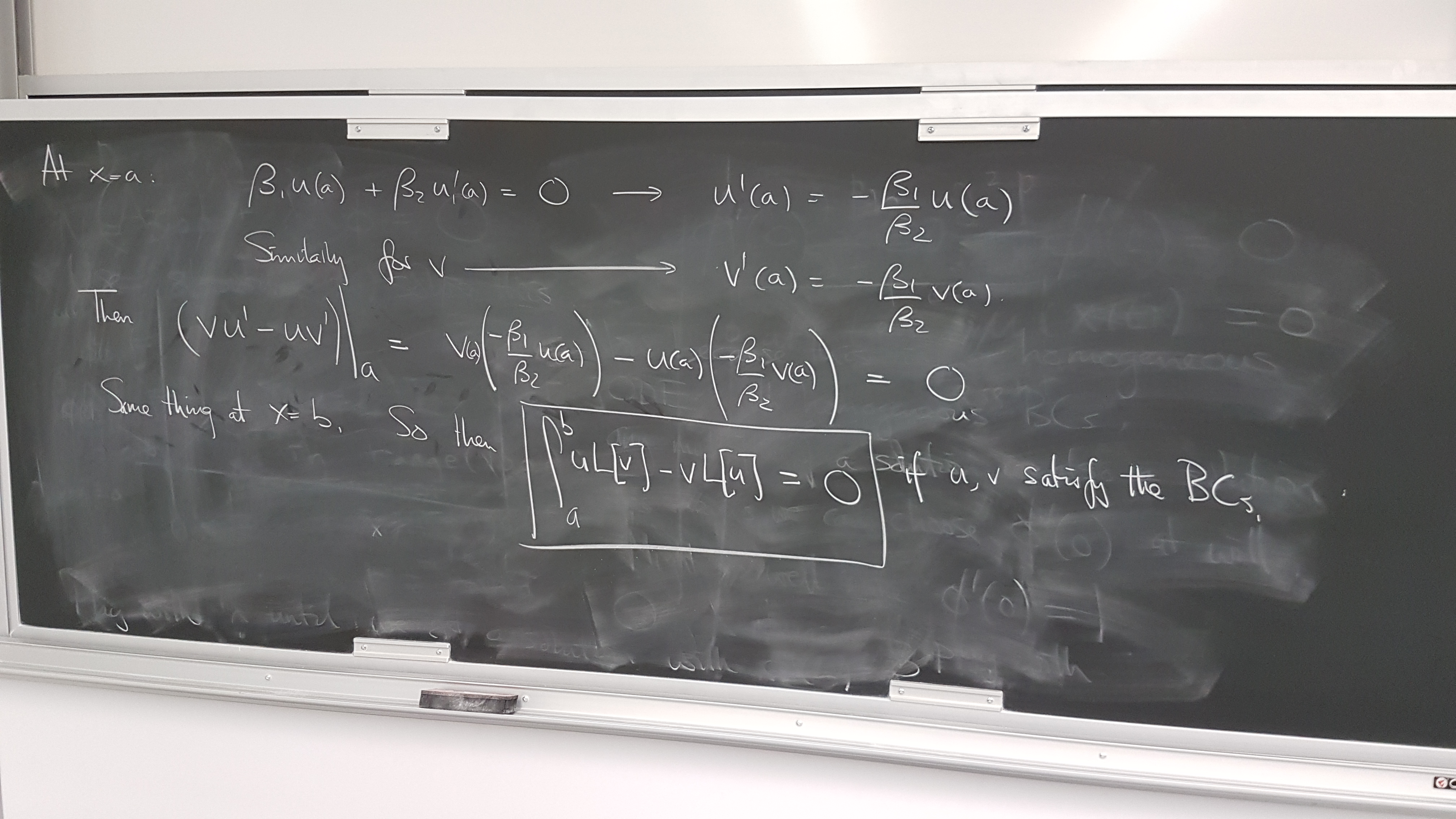
Eigenfunctions are orthogonal
in a slightly generalized sense
There is only one eigenfunction for each eigenvalue
up to multiplication by a constant
Back to our non-uniform bar
Can we verify that the eigenfunctions mutually orthogonal?
Can we also check to see if your eigenfunctions are orthogonal? (Just one pair, let's say.)
We will see that we actually have to modify the definition of orthogonality slightly to make this work:
∫L0φ1(x)φ2(x)σ(x)dx = 0
where σ(x) is a weighting function specific to the DE we're solving.
If we have two eigenfunctions and the weighting function all evaluated at a grid of x-values (the same grid for all), then the integral of their product can be approximated by forming the elementwise product of the three vectors and summing.
Note on checking orthogonality: We are computing approximations to the eigenfunctions, so they cannot be expected to be exactly orthogonal. So when we compute the (weighted) integral of their product, which you expect to be zero, you have to have some sense of how small is close enough to zero. Whatever this measure is, it should account for the fact that eigenfunctions are determined only up to scale. Thus your measure of their (lack of) orthogonality should be invariant (unchanged) if either of the eigenfunctions is rescaled. One way of doing this is to normalize all your eigenfunctions (analogous to making them "unit vectors") as follows:
φ(x) → (φ(x))/(√(∫L0φ(x)2σ(x)dx)).
Then if the "scalar product"
∫L0φ1(x)φ2(x)σ(x)dx
is small compared to 1, φ1 and φ2 can be considered approximately orthogonal.