2.3.X

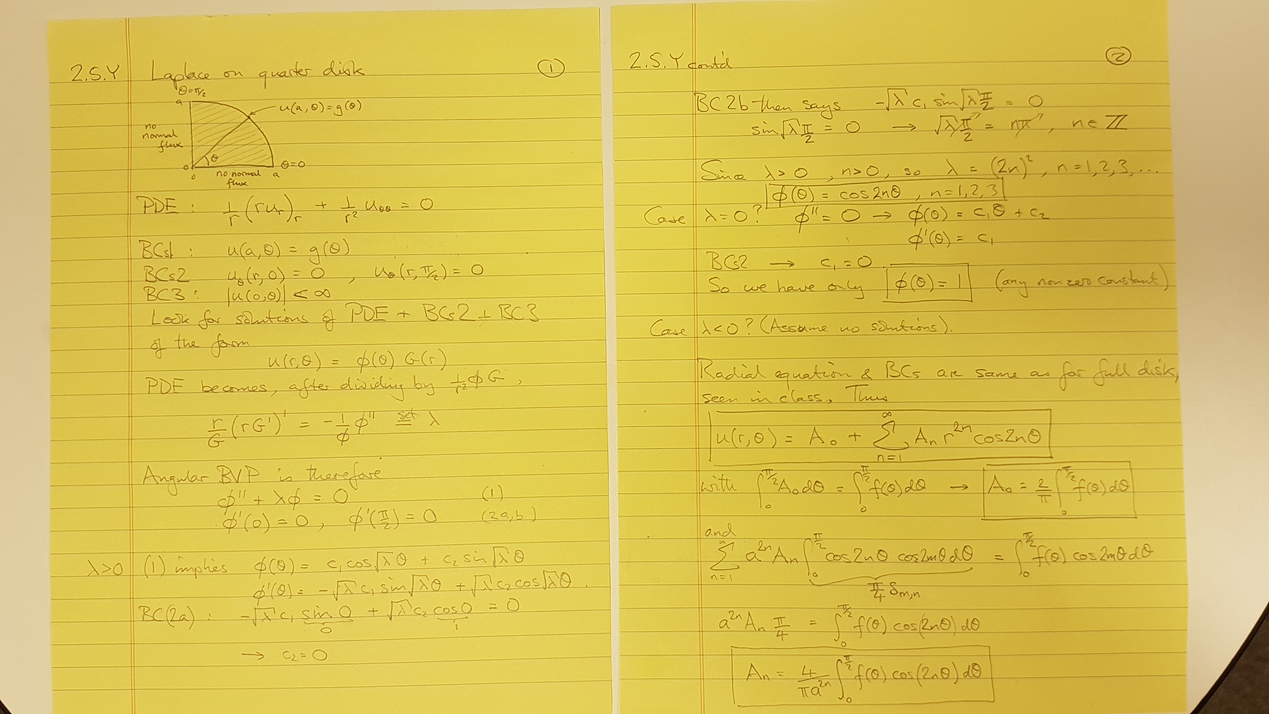
a. Make a plot of the solution of the heat equation for a laterally insulated copper bar of length 0.6 meters (2 ft), whose ends are maintained at 0 degrees, and whose entire interior is initially at 100 degrees. Show only snapshots for t = 10, 60, 360 seconds. For your approximation, include terms of the series for n up to M = 100.

Recall that the computation I did in class assumed k = 1, which is not the case here.

[1pt code turned in]

[4pts modifications correct in first 4 lines of code below]

L = 0.6         # length of bar in meters
M = 100         # max n
k = 1.11e-4     # thermal diffusivity of copper (OK if a bit different - varies with temperature and type)
tvalues = [10,60,360]  # times of snapshots

x = linspace(0,L,201)
n = arange(1,M+1)
B = 200*(1-cos(n*pi))/(n*pi)
for t in tvalues:
         Q = (B*sin(outer(x,n)*pi/L))*exp(-(n*pi/L)**2*k*t)
         u = Q.sum(axis=1)
         plot(x,u,alpha=0.5,label='t='+str(t))
xlabel('x')
ylabel('u(x,t)')
legend(loc='lower center');

[2pts image turned in]

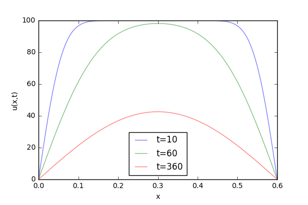
2. Run your code again for the case where the bar is stainless steel ("310") rather than copper.

[1pt for ok value of k]

L = 0.6         # length of bar in meters
M = 100         # max n
k = 4.2e-6      # thermal diffusivity of stainless steel 310 (OK if a bit different - varies with temperature and type)
tvalues = [10,60,360]  # times of snapshots

x = linspace(0,L,201)
n = arange(1,M+1)
B = 200*(1-cos(n*pi))/(n*pi)
for t in [10,60,360]:
         Q = (B*sin(outer(x,n)*pi/L))*exp(-(n*pi/L)**2*k*t)
         u = Q.sum(axis=1)
         plot(x,u,alpha=0.5,label=str(t))
xlabel('x')
ylabel('u(x,t)')
legend(loc='lower center')
savefig('2.3.Xb.png');

[2pts image turned in]

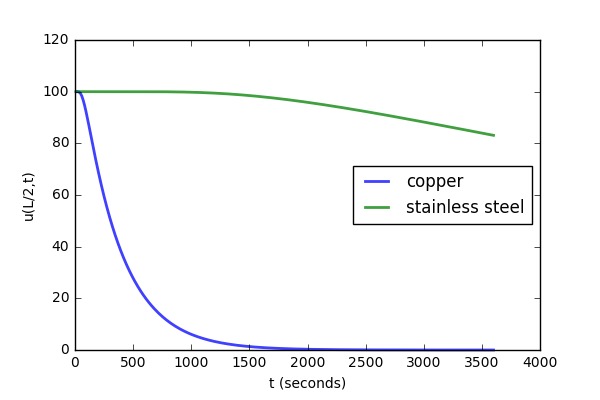
Comment on the difference. [2pts]

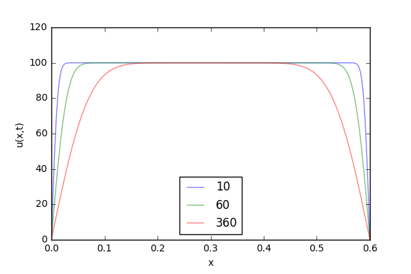
Wow! Stainless steel conducts heat very poorly compared to copper!

That explains why there are stainless steel pans with a copper bottom
to distribute the heat from the flames:

c. How long does it take for the temperature at the middle of the bar drop "noticeably" below 100 degrees? (Both materials.) I intend that you do this simply by re-running the code you used for parts a and b for various t-values that you choose by trial and error. This is an imprecisely posed question: any reasonable interpretation acceptable.

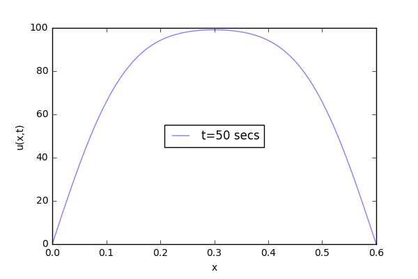
I will just use the same code as for (a) and (b) and fiddle with the t-value ...

Answer: For copper, at around 50 seconds you can start to see a gap
between the curve and the top of the plot.

[2pts for correct answer for copper]

[2pts for support of answer, such as a plot like the one below]

L = 0.6         # length of bar in meters
M = 100         # max n
k = 1.11e-4     # thermal diffusivity of copper (OK if a bit different - varies with temperature and type)
tvalues = [50]  # times of snapshots

x = linspace(0,L,201)
n = arange(1,M+1)
B = 200*(1-cos(n*pi))/(n*pi)
for t in tvalues:
         Q = (B*sin(outer(x,n)*pi/L))*exp(-(n*pi/L)**2*k*t)
         u = Q.sum(axis=1)
         plot(x,u,alpha=0.5,label='t='+str(t)+' secs')
xlabel('x')
ylabel('u(x,t)')
legend(loc='center')
savefig('2.3.Xci.png');

[1pt for correct answer for stainless steel]

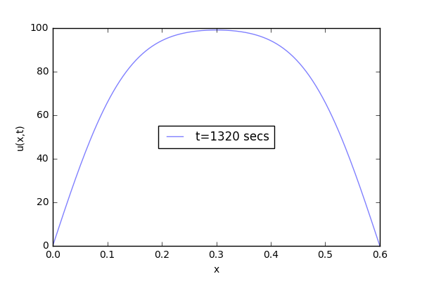
For stainless steel, you have to wait about 22 minutes! before you start to see a drop in temperature at the midpoint!

[1pt for support of answer for stainless steel]

L = 0.6         # length of bar in meters
M = 100         # max n
k = 4.2e-6      # thermal diffusivity of copper (OK if a bit different - varies with temperature and type)
tvalues = [22*60]  # times of snapshots

x = linspace(0,L,201)
n = arange(1,M+1)
B = 200*(1-cos(n*pi))/(n*pi)
for t in tvalues:
         Q = (B*sin(outer(x,n)*pi/L))*exp(-(n*pi/L)**2*k*t)
         u = Q.sum(axis=1)
         plot(x,u,alpha=0.5,label='t='+str(t)+' secs')
xlabel('x')
ylabel('u(x,t)')
legend(loc='center');
savefig('2.3.Xcii.png');

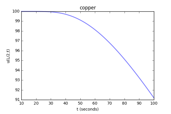
Make a plot of the temperature at the mid-point versus time. [Extra credit 4pts]

# copper
L = 0.6
M = 100
k = 1.11e-4 # thermal diffusivity of copper  #4.2e-6 # thermal diffusivity of stainless steel 310
x = L/2
n = arange(1,M+1)
B = 200*(1-cos(n*pi))/(n*pi)
t = linspace(10,50000,100)
t = linspace(10,100,100)
spacepart = B*sin(n*pi*x/L)
timepart = exp(-outer(k*t,(n*pi/L)**2))
spacepart.shape,timepart.shape
Q = spacepart*timepart
u = Q.sum(axis=1)
#print(Q)
plot(t,u,alpha=0.5,lw=2,clip_on=False)
xlabel('t (seconds)')
ylabel('u(L/2,t)')
title('copper');

# copper and stainless steel together
L=0.6
M = 100
x = L/2
tarray = linspace(10,3600,300)
k = 1.11e-4 # thermal diffusivity of copper
u = [sum([200*(1-cos(n*pi))/(n*pi)*sin(n*pi*x/L)*exp(-(n*pi/L)**2*k*t) for n in range(1,M+1)]) for t in tarray]
plot(tarray,u,alpha=0.75,lw=2,clip_on=False,label='copper')

k = 4.2e-6 # thermal diffusivity of stainless steel 310
u = [sum([200*(1-cos(n*pi))/(n*pi)*sin(n*pi*x/L)*exp(-(n*pi/L)**2*k*t) for n in range(1,M+1)]) for t in tarray]
plot(tarray,u,alpha=0.75,lw=2,clip_on=False,label='stainless steel')

xlabel('t (seconds)')
ylabel('u(L/2,t)')
legend(loc='center right')
savefig('2.3.Xcxii.png');

2.5.X

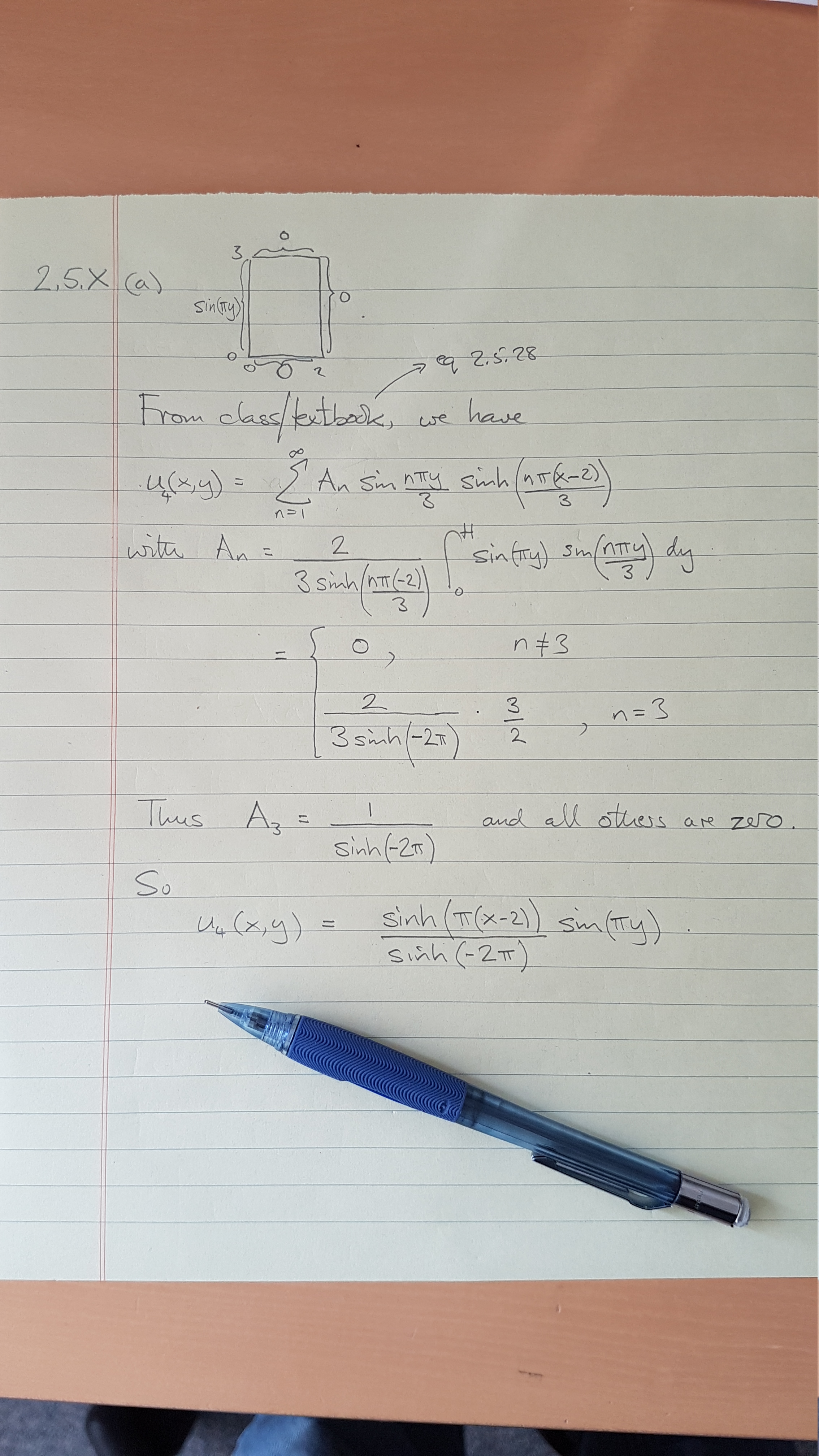
a. Solve Laplace's equation on the rectangle 0 ≤ x ≤ 2 0 ≤ y ≤ 3 with u = 0 on the boundary except for the side with x = 0 where u(0, y) = sin(πy).

[5pts]

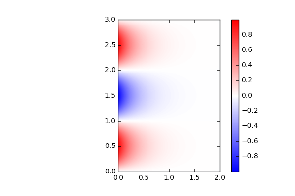
b. Make a picture of your solution by slightly modifying the following code:

[4 points for turning in code with correct modifications to 4 lines with #####]

from numpy import *
%matplotlib inline
from matplotlib.pyplot import imshow, savefig, colorbar

xmin,xmax = 0,2   #### x boundary values
ymin,ymax = 0,3   #### y boundary values
nx,ny = 200,300   #### number of points should be in proportion to length of axes

x,y = meshgrid( linspace(xmin,xmax,nx), linspace(ymin,ymax,ny) )

u = sinh(3*pi*(x-2)/3)/sinh(3*pi*(0-2)/3)*sin(3*pi*y/3)     ######## this is the solution
# or, more simply, u = sinh(pi*(x-2))/sinh(-2*pi)*sin(pi*y)

imshow(flipud(u),interpolation='bilinear',cmap='bwr',extent=[xmin,xmax,ymin,ymax])
colorbar()
savefig('2.5.Xb.png')

[2pts for turning in correct image]

2.5.Y

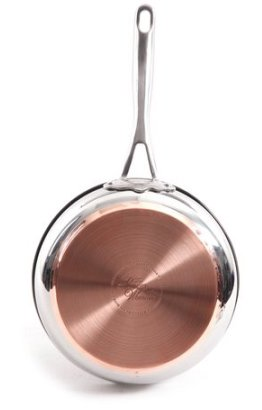
Solve Laplace's equation for u(r, θ) on the quarter-disk 0 < r < a, 0 < θ < (π)/(2) subject to boundary conditions u(a, θ) = g(θ) and no normal flux on the straight sides (θ = 0 and θ = (π)/(2)). I will show you a similar problem in class on Thursday.

[6 pts]