1.2

1.2.3 (derive heat equation for rod of varying cross-sectional area)

1.2.6 Grad students only

1.3

1.3.1, 1.3.2 (Show your work!*)

*Note that answers to starred exercises are in the back of the book.

1.4

1.4.3

1.5

1.5.3, 1.5.12

2.2

2.2.4 (Linearity) (a) [2pts] (b) [1pt]

2.3

2.3.2 (d) (Heat equation with prescribed temp at one end, no flux at the other) λ > 0 [4pts], λ = 0 [1pt ], λ < 0 [2pts].

2.3.5 (Show orthogonality of sines.) [4pts]

2.3.X Show that sinasinb = (1)/(2)[cos(a − b) − cos(a + b)] using Euler's formula. [3pts]

2.3.7 (Heat equation IBVP with no-flux boundary condtions.) (a) [1pt], (b) λ > 0 [3pts], λ = 0 [2pts], λ < 0 [2pts], (c) [1pt], (d) [3pts], (e) [1pt].

2.3.8 Grad students only. (Heat equation IBVP with lateral loss of heat.) (a) [3pts] (b) [4pts] Conclude with a sentence describing the effect of the lateral heat loss on the eigenvalues. [2pts]

2.3

2.3.X

a. Make a plot of the solution of the heat equation for a laterally insulated copper bar of length 0.6 meters (2 ft), whose ends are maintained at 0 degrees, and whose entire interior is initially at 100 degrees. Show only snapshots for t = 10, 60, 360 seconds. For your approximation, include terms of the series for n up to M = 100.

Recall that the computation I did in class assumed k = 1, which is not the case here.

b. Run your code again for the case where the bar is stainless steel ("310") rather than copper. Comment on the difference.

c. How long does it take for the temperature at the middle of the bar drop "noticeably" below 100 degrees? (Both materials.) I intend that you do this simply by re-running the code you used for parts a and b for various t-values that you choose by trial and error. Extra credit: make a plot of the temperature at the mid-point versus time.

2.5

2.5.X

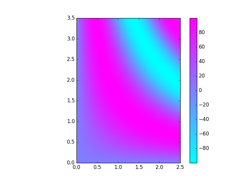
a. Solve Laplace's equation on the rectangle 0 ≤ x ≤ 2 0 ≤ y ≤ 3 with u = 0 on the boundary except for the side with x = 0 where u(0, y) = sin(πy).

b. Make a picture of your solution by slightly modifying the following code:

from numpy import *
from matplotlib.pyplot import imshow, savefig, colorbar

xmin,xmax = 0,2.5
ymin,ymax = 0,3.5
nx,ny = 250,350

x,y = meshgrid( linspace(xmin,xmax,nx), linspace(ymin,ymax,ny) )

u = 100*sin(x*y)

imshow(flipud(u),interpolation='bilinear',cmap='cool',extent=[xmin,xmax,ymin,ymax])
colorbar()
savefig('temp.png')

2.5.Y

Solve Laplace's equation for u(r, θ) on the quarter-disk 0 < r < a, 0 < θ < (π)/(2) subject to boundary conditions u(a, θ) = g(θ) and no normal flux on the straight sides (θ = 0 and θ = (π)/(2)). I will show you a similar problem in class on Thursday.

3.2

At points of discontinuity, use open circles for a limit point that is not included, and filled-in circles for the actual value there.

3.2.1 b,d,f Sketch the Fourier series on the interval -3L to 3L.

3.2.2 e Sketch the Fourier series on the interval -3L to 3L.

3.2.4

3.3

3.3.1 c Sketch all the series on the interval -3L to 3L.

3.3.2 c. Additionally use Python to make a picture of the 100th partial sum of the sine series. (See Day 11 notes. You need only the delete key, I think!)

4.2

4.2.1 (Wave equation for string sagging under gravity.)

4.4

4.4.1 Note that for part (b), the right end isn't "free" in the sense of being completely untethered. Think of it as being attached to a frictionless vertical rail.

4.4.3 (When you come up with a hulking collection of constants that will appear over and over again, give it a name so you don't have to write it more than once or twice!)

4.4.7 (Solution as two travelling waves.) Comment: I did not find it necessary (or helpful) to use either of the hints supplied in the book. You can just find out what properties of F are required for the given formula to satisfy all parts of the IBVP.

4.4.9 (Conservation of energy.)

Scoring

5.3.3 6pts

5.3.5
a 2pts
b 2pts
c 1pt
d 2pts

5.4.X

getting a good enough approximation of lambda: 2 pts
showing how they zeroed in on the answer: 2pts
presenting a graph of the eigenfunction with zero derivative at x=20: 2pts

5.5.1c  3pts

5.6.1a

correct specialization of RQ for this problem: 2pts
choosing a trial function that satisfies the BCs and computing the RQ: 2pts
doing the same for another valid trial function: 2pts

5.3

5.3.3 (Gerneral 2nd order ODE to Sturm-Liouville form.)

5.3.5 (Verifying that SL properties are true for a particular BVP where we know all the eigenstuff.)

5.4

5.4.X Use this code along with trial-and-error to find the third smallest eigenvalue of the non-uniform bar heat flow problem we have considered in class. Also make a plot of the corresponding eigenfunction. Determine λ₃ accurately enough that |φ^′(20)| (which should be exactly 0) is no bigger than .001.

5.5

5.5.1c (Show a SL problem is "self-adjoint".)

5.6

5.6.1a (Estimation of eigenvalue with Rayleigh Quotient.)

7.X

7.X.1

a. Make a plot of the spectrum of the low piano note recording in the Day 20 notes, and create a table of the frequency and amplitude of the principal peaks (as done in class for the brass bar on Day 20). Use the appropriate Python code from Day 20.

If you wish to use Jupyter notebook, just copy and past the code in, and change the 4th line to

wav = 'piano_low_f.wav'

NOTE: How to get interactive plots on Windows and Mac

b. Make a wav file of a signal that has sine wave components with exactly the frequencies and amplitudes you found in part a. Use the appropriate Python code from Day 20. Upload your wav file to UBlearns.

c. Comment on the similarity or dissimilarity of your synthesized sound and the original recording.

Upload a single plain text file with the two lines of your code with the frequencies and amplitudes (for part a) as well as your answer to c.

Office hour Wed 5-6:15pm as usual.

8.2 and 3

8.3.7 You are asked to find the evolution of the temperature distribution in a rod when one end is kept at 0 degrees, and the temperature at the other end is raised linearly with time. I'm going to structure the problem for you as follows ...

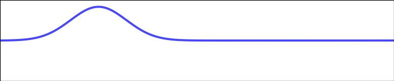
a. Before you do any computations or look up the answer in the back of the book, hand-draw a qualitative sketch of what you think the temperature distribution will look like as a function of x at some time T after the temperature-raising has been going for a while. Your answer will look like the picture below except yours will have a curve drawn in it.

b. Begin the calculation by making the BCs homogeneous in the simplest possible way: by subtracting off a function of x and t that is linear in x. Obtain the IBVP for the deviation v(x,t).

c. Find the eigenfunctions for the problem you obtained in part (b), and use them to obtain the time-dependent coefficients a_n(t) in the eigenfunction expansion of the solution of the IBVP. Compute the integrals so as to an obtain explicit (non-integral) formula for the general coefficient a_n(t) in terms of n and t.

d. What happens to your coefficients a_n(t) after a long time, i.e., as t → ∞? Make a plot of the partial sums of your solution for very large t by finishing the following code:

%pylab inline
L = 2
def a(n): return ########### your formula for a_n at infinite t here
def phi(n,x): return ######### your formula for phi_n(x) here
x = linspace(0,L,300)
v = zeros_like(x) # start with 0 all the way across
N = 20  # this is probably enough terms to get very close
for n in range(1,N):
          v += a(n)*phi(n,x)  # add the nth term to the partial sum
          plot(x,v,alpha=0.1) # plot the partial sum quite transparent so we'll see where it accumulates
ylabel('v(x,large t)')
xlabel('x')

Recall that ** is the exponentiation (power) operator in Python.

e. Find the equilibrium solution of your PDE for v subject to the BCs you obtained for v.

f. How is your equilibrium solution related to the plot you made in part (d)? Explain and/or demonstrate.

g. Re-do the eigenfunction expansion problem (finding u(x,t) analogously to what you did in part (c)) by defining w(x, t) = v(x, t) − v_E(x) where v_E(x) is the equilibrium solution you found in part (d), and solving the IBVP satisfied by w(x, t).

h. Was it worth the effort of refining the "offset" v to w in this problem? Justify your answer briefly (one sentence).

Scoring

For HW8 (Problem 8.3.7) please award points as follows.

a.
2 points for a curve that is concave up starting at (0,0). 1 point for any other curve that starts at (0,0) and ends at higher u for x=L.

b.
4 points (4 components of IBVP for v)

c.
6 points for correctly finding the differential equation satisfied by a_n(t)
1 point for the initial values a_n(0)  (all zero).
4 points for correctly solving the ODE for a_n(t).

d.
2 points for infinite-t limit of a_n(t).
4 points for display of correct code and plot.

e.
4 points for correct derivation of v_E(x).

f.
2 points for saying the two things are the same and some reasonable supporting statement or plot

g.
2 points for correct PDE for w.
4 points for correct coefficients.
2 points for correct solution u(x,t).

h.  1 point for any sensible comment.

9.3

9.3.9

In part (a), choose your two solutions of the homogeneous equation such that one satisfies the left BC and the other satisfies the right BC. Verify that they are linearly independent by showing directly that c₁u₁(x) + c₂u₂(x) = 0 for all x implies c₁ = c₂ = 0. (You will need the assumption that L is not an integer multiple of π.)

x. Make a plot of the Green's function G(x, x₀) for L = 3 and (i) x₀ = 2 and (ii) x₀ = .2.

9.5

9.5.11

Note: this is very similar to the example worked out in class Day 24. Here is a hint: the Green's function for the example in class is pictured here:

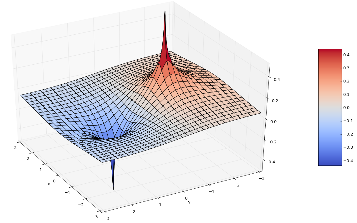
and the Greens's function for this homework problem is pictured here:

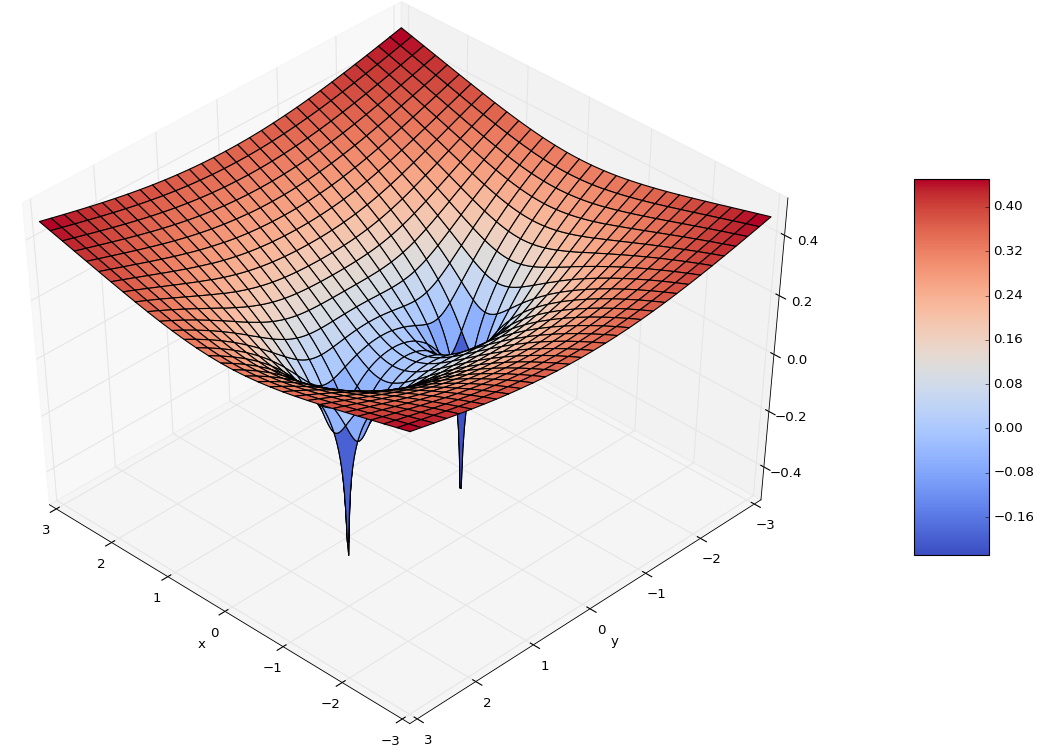
See how the value is 0 along the x-axis in the upper picture, while the y-derivative is 0 along the x-axis in the lower picture.

Hint for part (b): the key equation is the (un-numbered) one above Eq. 9.5.46 on p421.

Ch 12

X1. Solve the problem xu_x + (x + y)u_y = 7 with u(1, y) = 3y for 0 ≤ y ≤ 1, and describe the region over which the solution is uniquely determined.