MTH 306 First Projects, Spring 2025
Contents
The big picture
In each of the 3 project options you have a mathematical model (or several) of something in the real world. The models are differential equations. The purpose of the project is to test the model(s), by comparing their predictions with your own real-world observations.
Note: For each project I have created a UBx question to allow you to check your solution of the differential equation(s), so that you can have confidence in proceeding with it.
OPTIONS
You will work in teams of 4. Your team will choose one of the 3 options below. There will be approximately the same number of teams working on each option.
Everyone should understand and participate in every aspect of the project.
(1) Draining cone
See if you can accurately predict how water drains out of a cone made of a rolled-up overhead transparency with a small opening at the vertex. Torricelli (1608-1647) used a simple idea to come up with a "law" for how fast a fluid drains from a container with a hole in the bottom: he imagined the exit speed of the fluid would be the same as if the exiting fluid had fallen freely from the height of the top surface of the fluid. This (possibly dubious) principle leads to the equation
where y is the depth of the fluid at time t, A(y) is the top surface area of the fluid, b is the area of the exit hole, and g is the local acceleration due to gravity = 9.81m ⁄ s2. (The LHS is the volume of fluid exiting per unit time.) See if Torricelli was close to being right. First get your experimental measurements. Then solve the differential equation to predict how it drains and compare the theoretical draining curve (depth y vs. time t) with the experimental one. I'll provide some transparency sheets for you to make a cone with.
You can do the timing and measuring any way you think will work well. My recommendation is to attach a ruler to the outside of the cone, and make a video of the draining process with your phone. (You'd have to do a little trig to convert the tilted ruler readings to vertical heights.) See below for code to extract individual frames from a video, if that's helpful.
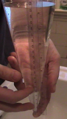
I recommend you use quite a small exit hole, so that the times are long and easy to measure accurately, although this makes accurately determining b tricky. If the exit hole is small, you can ignore the truncation of the cone in your formula for A(y), i.e. you can take y=0 as corresponding to the vertex of a cone.
Caution: be sure not to confuse the time it takes to drain to depth y with the time it takes to drain completely from depth y.
Do not be afraid of saying the model is poor if that's what your data shows.
(2) Falling filters
What is the right law of air friction? In some places you may read that air friction is proportional to the velocity, and other places say it's proportional to the square of the velocity. The goal of this project is to see which model works better for falling stacks of coffee filters. Newton's law of motion for a dropped object is
where M is the mass, g is 9.8m ⁄ s2, v is the downward velocity, and f is the air-friction force, which we believe depends only on velocity.
Get hold of 15 coffee filters (I have a box of them).

Find a (wind-less) place where you can drop the filters from some measured height (at least 1 meter, maybe several meters), and time how long it takes a stack of 1, 2, 4, and 8 filters to hit the ground.
See if you can determine whether f(v) = k1v or f(v) = k2v|v| is a better model for the frictional force. (Note v|v| = v2 if v is non-negative, as it will be in this project.) The k in each case is a constant specific to the coffee-filter shape that you don't know in advance, but that you assume is very close to the same for 1, 2, 4, and 8 filters stacked together, because the geometry is very close to the same in all cases. You should solve the differential equation to get v(t) and then from that get the height y(t) for each version of f , and each number of filters.
You can do the timing and measuring any way you think will work well. What I did was take a video of the filters landing and then examine individual frames of the video (see below for code to generate them) to find the times at which each of the stacks hit the ground. Knowing the time at which they were dropped (use audio track of video?) you can determine the duration of the fall for each stack of filters.
Once you have your experimental times for each of the 4 objects to fall some number of meters, you can plug those times into your solutions of the differential equations for y(t) and see how well you can get those y(t) to match the actual distance the filters fell - by adjusting the constants k1 and k2 respectively.
If, hypothetically, after adjusting k1 and k2 to get the best fits possible, you had this result:
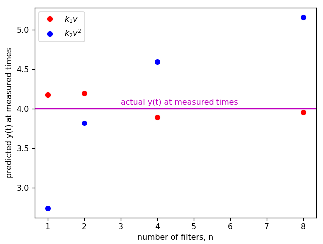
you would conclude that the k1v model is better.
Note that once you've solved the DE for v(t), you can obtain y(t) by just integrating. Also, in case it's of any use to you: integral of 1 ⁄ (a2 − x2) is arctanh(x ⁄ a) ⁄ a , and the integral of tanh(bx) is log(cosh(bx)) ⁄ b.
Hint: I would set M = nm where n is the number of filters, and m is the mass of 1 filter, and then use the parameters r1 = k1 ⁄ m, r2 = k2 ⁄ m as my adjustable parameters.
(3) Hanging chain
Some simple ideas about mechanical equilibrium lead to a prediction that the shape of a hanging chain should obey the differential equation
where x is the horizontal coordinate, y is the height of the chain above some arbitrary reference level, and a is a constant that depends on how much length of chain you have between the two support points. Other properties of the chain, like its density, are predicted to be irrelevant. Note that if we call s = (dy)/(dx) (for "slope"), this differential equation is a first order separable equation in s, and then y could be obtained from s just by integrating. However ... here is a major time-saving hint: this is a case where you will probably get to a tidy solution formula faster by trial-and-error: look up the hyperbolic functions - their derivatives and the relationships among them.
See if the this model accurately predicts the shape of an actual hanging chain. Find some kind of chain (a necklace, a bicycle chain, ...), support its ends at some points on a wall and carefully record the shape of the arc of the chain by taking a photograph. Note: to minimize distortion, the camera should ideally be several times as far from the chain as the extent of the chain. You could take a test picture of a tiled floor to see how much distortion your camera introduces.
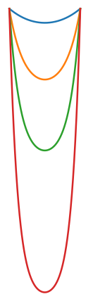
Your solution of the differential equation will contain several adjustable parameters (a, and two constants of integration). Choose at least two chain shapes, from "long" to "short" (as in the pictures on the left below). See if the solutions of this differential equation predict a shape that's closer to reality than some arbitrary other curves like a parabola or an ellipse. A challenge in this project may be in choosing the adjustable parameters so as to optimally match the shape in the photo.
In this project, because the differential equation is nonlinear, a vertically or horizontally stretched shape of a chain not actually the shape of a chain (though it looks quite like one). Therefore it is essential that any plots you make for comparison with a real chain have the same scales on the horizontal and vertical axes (units per cm): see the code below which also shows how to load your photo and how to plot a curve on top of it.
Modified instructions to see coordinates of mouse pointer because "%matplotlib notebook" and "%matplotlib ipympl" seem to be broken in the latest version of Jupyter. We need to run this code from the terminal or Anaconda Prompt, similarly as in Lab 6. Go to your Jupyter Home page, click New ... and choose New File. Name the file something.py. Then double-click the filename and paste the following code into the file and Save it.
from resources306 import *
from PIL import Image
img = np.asarray(Image.open('20250226_135241_chain.jpg')) # load image (change this to your own image)
img = np.transpose(img,(1,0,2)) # my image needed to be rotated - delete this line if not needed
w,h,d = img.shape
plt.figure( figsize=(3,4) ) # can make figure any size you like
plt.subplot(111,aspect=1)  # ensure vertical and horizontal scales are the same
x = sp.symbols('x')
expressionplot( 3300 - 4000*(x-1500)**2/1500**2, x, 200,2800, color='yellow', alpha=0.6) # your own formul
plt.imshow(img,extent=(0,h,0,w))
plt.show()
Then run the code by typing "python something.py" in the terminal or Anaconda prompt. You may need to first use the command "cd" (change directory) to move to the folder where you created the .py file. Something like:
cd "My 306 Project"
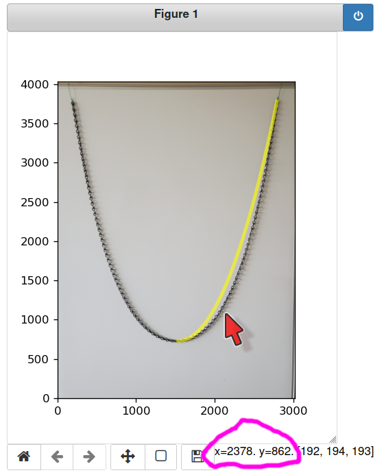
Note that the above plot shows that a parabola provides a poor fit to the shape of the chain. The solution of the differential equation is NOT a parabola. Also note that a rope is not a chain: a chain does not resist bending at all.
Instructions for writing your Report
Individual Project Diary
In addition to writing a team Report collaboratively with your team members, you must keep and eventually turn in your own personal diary of your work on the project. Each entry should have date, start time, end time, what you did, who you did it with. Turn this in separately from your report. This should be done as you go, not retrospectively at the end. I may ask you to turn a snapshot of this prior to the project due date. You should write your diary independently of your teammates.
Team report
You will write and submit your team's report as a Jupyter notebook.
When you write it, imagine your are writing to a classmate who is familiar with the course material, but has no specific knowledge of your topic.
Use carefully labeled and described illustrations if and where appropriate. Use Python to generate any plots that you include - see below for help on this.
Write as clearly as you can, in complete and grammatically correct sentences (including those sentences that contain equations, software commands, etc.).
Four screens is too short. Twenty screens is probably too long.
Required sections of report
Introduction
Set the stage for your reader. Briefly describe what your project is about. State the goal of your project.
Description of experiments, and analysis of model differential equations
Complete and careful description of the experiments you performed, and of your analysis of the differential equation model(s).
Comparison of experiment and theory
Careful comparison of the model predictions and the experimental results. Try to account for any discrepancies.
Conclusions
Summarize the things you have learned about your subject matter and about differential equations in general. State the "take-home message" of what you've done.
Runnable code
You must include all your Python code in your report, either in the body of your report or as an Appendix, and in a form that allows me to run it without any editing.
Cautions
Don't misrepresent anything! You can get an A+ for a carefully done project even if the model turns out to be not good. If your results turn out to be inconclusive, say so clearly, and suggest how the experiment/model/comparison could be improved.
Check all analytical solutions by plugging them back into the differential equation. I have provided solution validators on UBx so that you can check your solution and then proceed in the confidence that it's correct.
Every picture must be properly integrated into the report.
GET HELP EARLY IF YOU NEED IT!
Creating a report in Jupyter Notebook
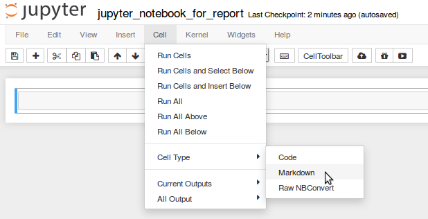
Set cell type to "Markdown" for non-code sections.
Math can be formatted like this, shown below in unrendered (left) and rendered (right) forms:
Code for extracting frames from a video
This code uses the module OpenCV a.k.a. cv2. If you get a message "no module cv2", you can install it using conda install -c menpo opencv
# adjust the next 4 lines according to your needs
video_file = 'myvideo.mp4'
start_time = 21   # seconds
stop_time  = 25   # seconds
myframefolder = 'myvideo_frames'

# no need to change anything below here
import cv2
video = cv2.VideoCapture(video_file)
frames_per_second = video.get(cv2.CAP_PROP_FPS)
print(f'{frames_per_second} frames per second')
from os.path import exists
from os import makedirs
if not exists(myframefolder): makedirs(myframefolder) # create folder for frames
start_frame = int(start_time*frames_per_second)
stop_frame =  int(stop_time*frames_per_second)
success = True
frame = 0
saved = 0
while success:
        success,image = video.read()
        if frame >= stop_frame: break
        if frame >= start_frame:
                cv2.imwrite(myframefolder+'/frame'+str(frame).zfill(5)+'.jpg',image)
                saved += 1
        frame += 1
        print(frame,end='\r')
print(f'Saved {saved} frames in folder {myframefolder}')
Basics of making plots
I'm demonstrating here just a few of the many many options that are available to create, adjust and decorate plots. You can Google to find more.
[Note to self: if use svg backend, plots are not embedded in the notebook. retina works nicely.]
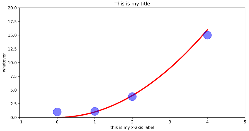
from resources306 import *
# The following line is not necessary, but I find this renderer makes better pictures than the default one:
%config InlineBackend.figure_format = 'retina'

xdata = [ 0, 1, 2, 4 ]
ydata = [ 1, 1.1, 3.8, 15. ]
plt.plot(xdata,ydata,'bo')

x = np.linspace(0,4,200) # 200 uniformly spaced points between 0 and 4
plt.plot( x, x**2, 'r' );
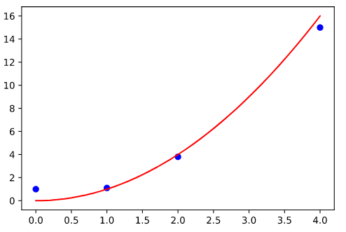
# Again, with some adjustments and decorations this time
plt.figure(figsize=(10,5))
plt.plot( x, x**2, 'r', linewidth=3 );
plt.plot(xdata,ydata,'bo',markersize=20,alpha=0.5)
plt.xlim(-1,5)
plt.ylim(0,20)
plt.xlabel('this is my x-axis label')
plt.ylabel('whatever')
plt.title('This is my title');
plt.savefig('myplot.png',bbox_inches='tight')
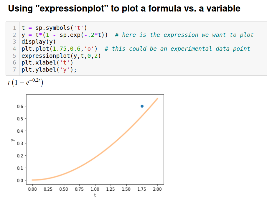
To plot a solution formula you can alternatively use expressionplot:
If you need the horizontal and vertical axes to have the same scale here's how:
plt.subplot(111,aspect=1)
plt.plot(xdata,ydata,'bo',alpha=0.5)
plt.plot( x, x**2, 'r' );
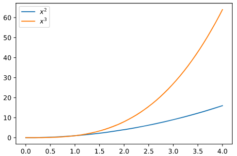
To label curves, you can use legend:
plt.plot(x,x**2,label='$x^2$')
plt.plot(x,x**3,label='$x^3$')
plt.legend(loc='upper left');