MTH 306C Spring 2024 Labs
Contents
- Lab 1, Wed, Jan 24
- Lab 2: Plotting slope fields and using them to solve IVPs
- Lab 3 (Feb 6, 2024): Euler's method to solve an IVP (step halving)
- Lab 4 (Feb 13): A model of a harvested fish population
- Lab 5 (Due to Exam on Feb 21, I think we'll postpone this to Feb 28): The most comfortable shock
- Lab 6 (March 6): The phase plane
- Lab 7: focus on Homework due March 13
- Lab 8: the TD diagram
- Lab 9: skyscraper dynamics
- Lab 10: Euler's method for systems
- Lab 11: Series solutions
- Lab 12: Building functions with the Heaviside step function
Lab 1, Wed, Jan 24
1. Get up and running with Jupyter and Python
Launch Jupyter Notebook from Anaconda Navigator, and open a new Python 3 notebook.
Check that 2+2=4:
2+2
Use Shift-Enter to execute the code in a cell.
To download the resources file for MTH 306, copy, paste, and run the following code in your Jupyter notebook.
import requests
r = requests.get('https://raw.githubusercontent.com/UBmath/306/master/resources306.py')
with open('resources306.py','w') as f: f.write(r.text)
The above needs to be done just once for the whole semester.
Check that everything is ok by running this code which plots the exponential function e − 2t for − 1 ≤ t ≤ 2:
from resources306 import *

t = np.linspace(-1,2,200)
plt.plot( t, np.exp(-2*t) )
plt.grid()
2. Enroll in UBx course for homework
Most homework will be done through the online system called learning.buffalo.edu, also known as UBx. (This is UB's instance of the Open edX platform.)
Here are instructions for registering and enrolling in the 306 course on UBx.
Lab 2: Plotting slope fields and using them to solve IVPs
Wednesday, Jan 30
(1) Start up Jupyter Notebook and open a new Python3 notebook.
(2) Import the resources306 module:
from resources306 import *
(3) Create a slope field plot for the differential equation
over the region where t runs from 0 to 5 and y runs from -1 to 5.
Here's code similar to what I showed you in class for a different DE, dy/dx = (y-x)/4:
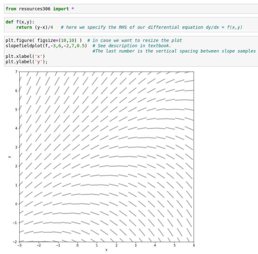
Notes:
(4) Tape a piece of paper that you can see through over the plot on your computer screen. If you don't have paper that's transparent enough, ask the TA for a sheet of tracing paper.
(5) On your slope field, sketch a curve with the following properties:
- it starts at t = 0, y = 0,
- its slope agrees with the slope field at every point along it.
(6) From your picture, estimate as accurately as you can y(4) if the function y(t) satisfies
y(0) = 0 and (dy)/(dt) = cosy + ysint
for all t between 0 and 4. Annotate your picture to show how you got your estimate. Take a photo of your work for your own future reference.
(7) Have the TA check the correctness of your work.
Lab 3 (Feb 6, 2024): Euler's method to solve an IVP (step halving)
This is to be done with students working side-by-side in pairs. Discuss and share!
The problem
If y(t) satisfies the differential equation dy/dt = cos y + y sin t, and additionally y(0) = 1, determine y(4.5) to an accuracy of ±0.005 using Euler's method (implemented in Python).
The method
Here is an implementation of Euler's method in Python, which I wrote and you can copy. Note that the particulars in the code below are different from those of the problem you're asked to solve: you'll need to adapt them to your problem.
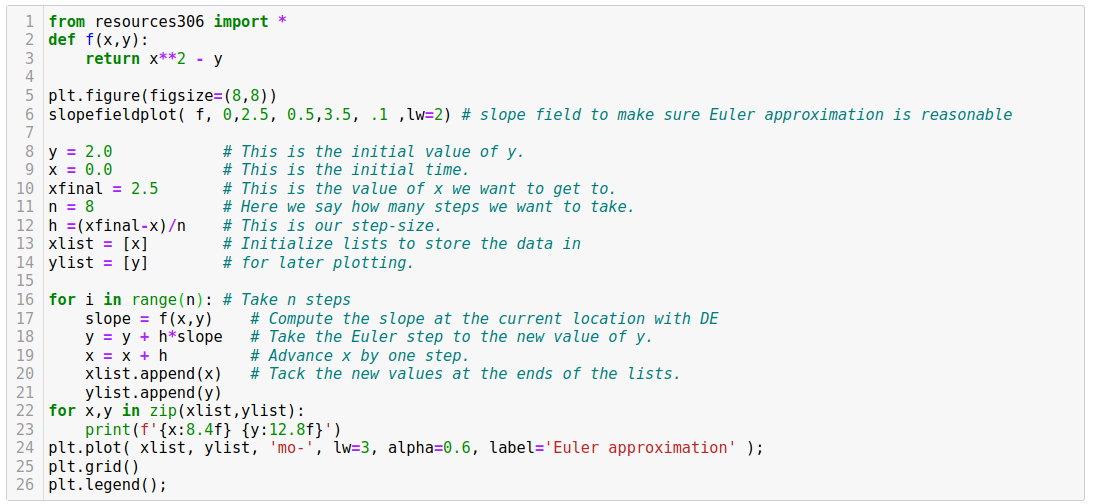
How to estimate the error
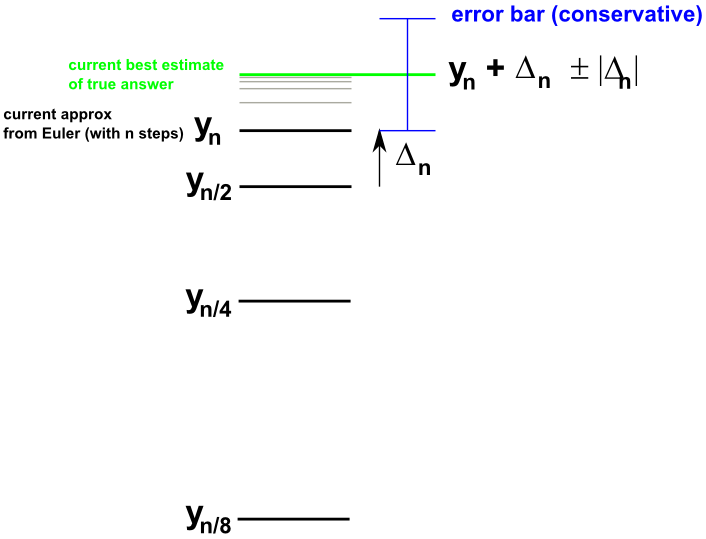
To get an estimate of the error in your Euler approximation, you can halve the step size and take the difference in your two approximations for y(4.5) as an estimate of the error of the better approximation. If that diffference is greater than 0.005, then you'll need to halve again, etc.
In a spreadsheet or on a piece of paper, make a table showing how your estimate of y(4.5) depends on the step size you use.
Write up your results in your Jupyter notebook. Your answer should look something like y(4.5) = 23.459 ± 0.002, or 23.456 < y(4.5) < 23.463 (but with different numbers). The best approximation to the exact answer (without doing more Euler runs) is your best Euler result (the one using the smallest steps) plus the difference between this result and the result with half as many steps.
Ask Nepa to check your work.
Lab 4 (Feb 13): A model of a harvested fish population
Note: this is very similar to a problem in Homework 4, due this Friday.
Here is a fish-population model incorporating the effects of
- fish not finding mates if the population is too small,
- the death rate going up as the population increases, and
- the population being harvested with "effort" e:
(dP)/(dt) = f(P) = P(1 − P)(4P − 1) − eP
P is the population size (number of fish). The parameter e, which might for example represent the number of boats allowed in the fishing fleet, is to be considered constant in time, but we'll be interested in various values for that constant.
(1a) Sketch the phase line for this equation when there is no fishing at all (e = 0). Use all you know about the graphs of cubic functions to help you. Or use Python to sketch the graph of f when e = 0.
Here's some code you could use:
from resources306 import *
P = sp.symbols('P')
plt.plot([0,1.1],[0,0],'k') # draw the horizontal P-axis
f = P*(1-P)*(4*P-1) - 0*P
expressionplot(f,P,0,1.1)  # draw f(P)
plt.xlabel('P')
plt.ylabel('f(P)',rotation=0);
(1b) Use your phase line to help you describe the possible things that can happen to the fish population in this case:
- in words (write them down)
- in a qualitative sketch of the solution curves: rotate your phase line vertical and use the horizontal axis for time.
(2a) Now figure out what happens when e is greater than 0. Start by thinking what the effect is on the graph of the RHS of the DE when you subtract eP first for tiny positive values of e, then for larger values. Use Python if you like, varying the value of e and seeing what it does to the graph of f.
(2b) Sketch the phase line for this equation when there is fishing with effort e = 1.
Use your phase line to help you describe the possible things that can happen to the fish population in this case:
- in words (write them down)
- in a qualitative sketch of the solution curves: rotate your phase line vertical and use the horizontal axis for time.
(3 ) The phase lines in parts 1 and 2 are qualitatively different. Try to illustrate how the phase line in 1 "morphs" into the phase line in 2, by drawing a sequence of phase lines side by side. (This is called a "bifurcation diagram").
(4 ) Is there a definite transitional case? If so, can you sketch the phase line for it in your bifurcation diagram, and even figure out the e-value where it occurs?
Lab 5 (Due to Exam on Feb 21, I think we'll postpone this to Feb 28): The most comfortable shock
NOTE TO SELF: In future, arrange to have Homework 5 due before this lab!
Background
In this lab you will explore the behavior of a vehicle that is moving along a flat road and then suddenly hits a ramp. You will examine the effect of the damping caused by the vehicle's "shock absorbers", and try to decide what is the best value for the damping coefficient.
If you think you might be pressed for time, you can skip straight to last sentence of this section and refer back to the preceding as needed.
A simple model of the response a car to unevenness of the road is
where y is the height of the car frame off above some reference level, h is the height of the road surface above that same reference level, and L is the natural (uncompressed) length of the shock absorber and wheel assembly. The shock absorber consists of a spring (with constant ks and a damper with constant kd.
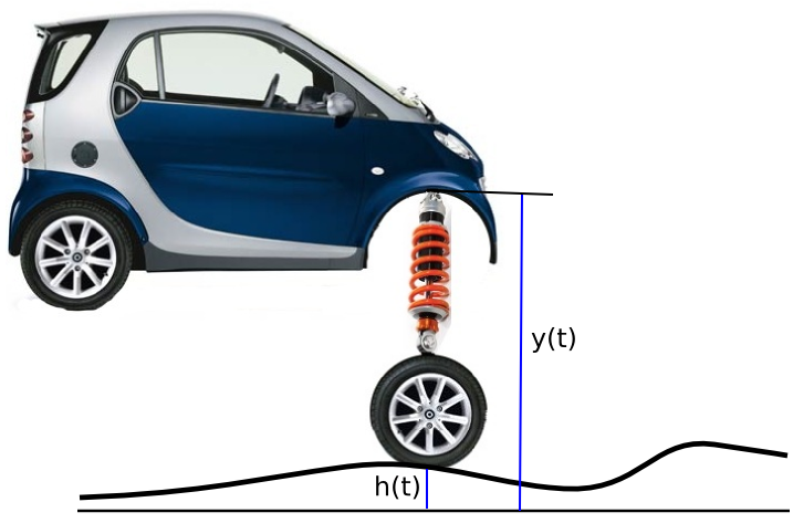
If you change variables, defining u(t) as y(t) minus the equilibrium value of y at the instantaneous value of h(t)
the differential equation (1) becomes
or, dividing through by m,
where 2p = kd ⁄ m and q = ks ⁄ m. Remember h(t) is the height of the road surface at the point right under the tire. 1. If a car is traveling on a perfectly flat road and then at time 0 hits a ramp that's inclined with slope, s,

then h''(t) is zero except for a very sharp spike at t=0. The effect of that spike is to instantaneously make u' = -s. Thus the motion after t=0 is governed by the IVP
This is a damped harmonic oscillator equation just as we have studied in class and the textbook section 2.4.3 (pp107-110).
Assignment
(1) Qualitatively, how does the response of the car to hitting the ramp differ for cases of high and low damping constant, p?
(2) Where is the cross-over between the two main types of behavior? I'm looking for an equation for p in terms of q, and then for kd in terms of ks and m.
(3) Fix the Python code below so that it has the correct formulas for the solution of the IVP (5) for all three of the cases: (i) underdamped, (ii) critically damped, and (iii) overdamped. (I have introduced several deliberate errors.)
def ivp_solution(p,q,s):

        # Return the solution formula for the IVP,
        #  u'' + 2 p u' + q u = 0,
        #  u (0)=0 , u'(0)=-s

# WARNING: THERE ARE SOME MISTAKES YOU NEED TO FIX

        pcrit = sqrt(q)

        if p < pcrit:
                alpha = -p
                beta  = sqrt( q**2 - p )                  # FIX THE MISTAKE IN THIS LINE
                u = -s/beta*exp(alpha*t)*sin(beta*t)
                print('Underdamped: alpha=',alpha,', beta=',beta)

        elif p > pcrit:
                r1 = -p + sqrt( p**2 - q )
                r2 = -p - sqrt( p**2 - q )
                u = (-s/(r1+r2))*(exp(r1*t)-exp(r2*t))    # FIX THE MISTAKE IN THIS LINE
                print('Overdamped: r1=',r1,", r2=",r2)

        else: # p == pcrit
                r = -p
                u = -s*t*exp(r*t)
                print('Critically damped: r=',r)

        return u

from sympy import sqrt,exp,sin,cos,diff,symbols
t = symbols('t')

u   = ivp_solution(2, 20, 1)
display(u)

up  = diff(u ,t)
upp = diff(up,t)
Note how we are using sympy's diff function to take the derivatives. The output will look like this:
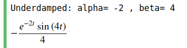
(4) What is the value of the acceleration experienced by the riders at t=0, the moment the car hits the ramp, in terms of p, q and s, in all three cases? (You can get this directly from the differential equation!) Comment on what your answer says about the comfort or discomfort of the passengers as a function of p (and s).
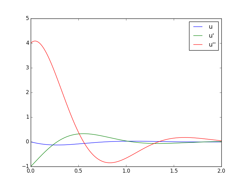
(5) Let s=1, q=20, and make plots of u, u', and u'' all versus t for high, medium, and low values of p. Use the code shown above as a starting point.
Here is some more help with Python for this task:
from resources306 import *
expressionplot(u,t,0,2,label="u")
plt.legend()
plt.grid()
(6) How should the spring constant ks and damping constant kd be chosen by the designers of the shock absorber? In terms of comfort for the riders, is there a disadvantage to having the damping too low? Is there a disadvantage to having the damping too high? What do you think is the optimal choice of damping constant, p, in relation to the critical value? Justify your answer carefully.
Lab 6 (March 6): The phase plane
(Printed copy of these instructions provided.)
In class on Monday we began our study of systems of differential equations. An example is that we have two functions x(t) and y(t) and the rate of change of each of them can depend on both of them.
To get familiar with the situation, today you will use a computer program to explore the relationship between the xy-plane picture ("phase plane" – like a phase line but 2D) and the graphs of the two dependent variables x and y versus time. Work in pairs so that you can discuss things with your partner as you go.
Keep a written record of what you do and discover.
Experiment
Copy and paste this text, phase_plane_draw_notebook.txt that I wrote for today's lab. When you run it, it allows you to draw curves in the xy-plane. While you do this, the program also draws corresponding plots of x(t) and y(t).
(1) Run the code, and in the phase plane panel, draw a circle clockwise, as smoothly as you can, starting at a point on the y-axis. Look at the graphs of x(t) and y(t) that you have generated. Do they make sense?
(2) How would the graphs of x(t) and y(t) differ if your starting point were on the x-axis? Predict what you think to your partner before trying it. Then check your prediction by doing it.
(3) How would the graphs differ if you drew the same circle, but slower? Again, predict first, then try it.
(4) How would the graphs differ if you drew the same circle, but you slow down dramatically for a short time while you're drawing the circle? Once again, predict first, then try it.
(5) How about if you draw the same circle but counterclockwise. Predict, then check.
(6 Draw some spirals and observe the corresponding graphs of x(t) and y(t).
(7) Test your visualization skills! Call over the TA. She will cover up the phase plane panel with a piece of paper and draw something while you're not looking. You will see only the graphs of x(t) and y(t). Your task is to figure out what is drawn on the xy-plane. Make a sketch before you look. When you're done, uncover the picture and sketch of what it really looks like beside your prediction. If you have time, give your partner some more tests of the same type.
(8) Write a couple of sentences about something you have learned from today's exercise. Turn in everything you've written today.
Lab 7: focus on Homework due March 13
Wednesday Mar 13
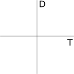
Lab 8: the TD diagram
This should all be done by hand, without using your computer, and without looking at the textbook or the internet.
The characteristic polynomial for the general 2x2 matrix
is
1. Expand it out, and rewrite it using the short-hand
D for ad − bc (the determinant of A),
T for a + d (the "trace" of A).
2. Use the quadratic formula to get an expression for the eigenvalues - in terms of D & T.
3. What is the sum of the two eigenvalues? What is their product? (Both in terms of D & T only.)
4. Under what conditions will we have distinct real eigenvalues? Make a sketch of the TD plane and shade the corresponding region.
5. Where in the TD diagram is the "Emily & Jacob" example?
6. Find an example of a nodal sink in your class notes and mark the corresponding point in the TD diagram.
7. Which region of the TD diagram corresponding to nodal sinks? Hint: how can you characterize two numbers being both negative in terms of their sum and their product? Shade this region using a different color/pattern than you used in Question 4.
8. Find an example of a saddle in your class notes and mark the corresponding point in the TD diagram. Indicate the region of saddles in the TD diagram.
9. Where are the nodal sources?
10. Indicate on your diagram where the spiral sinks and spiral sources are respectively.
11. Where in the diagram do the harmonic oscillators "live"? The harmonic oscillator equation is (d2y)/(dt2) + 2p(dy)/(dt) + qy = 0 with constants p ≥ 0 and q > 0, which you'll have to convert to a first order system in order to answer this question.
Turn in your work as part of this week's homework.
Wednesday Apr 3
Lab 9: skyscraper dynamics
Qualitative analysis of a nonlinear 2D autonomous system
No computers and no internet today. This should all be done by hand and brain.
A. The model
Here is a model of a swaying skyscraper in which y(t) represents the horizontal deflection of the top of the building. (This DE is called Duffing's equation.)
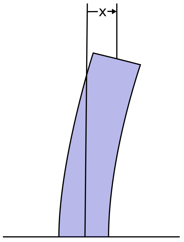
The model is actually just Newton's 2nd law of motion (F = ma, or a = F ⁄ m, where a is the acceleration d2x ⁄ dt2, m is the mass, and F is the total force), with 3 contributing forces:
(i) a frictional force proportional to the velocity.
(ii) a restoring force proportional to the deflection (due to the rigidity of the building), and
(iii) a force due to gravity which tends to pull the building over further when it's leaning,
1. Which force corresponds to which term in the DE?
B. Qualitative analysis
Your task: Describe the effect of blasts of wind of various strength which give the builidng a kick (i.e. give it a non-zero velocity at position x=0). Here are some steps that will assist you ...
2. Convert the 2nd order DE into a pair of 1st order DEs by defining a second dependent variable v as
3. Sketch the nullclines in the phase plane of your 2D autonomous system (x horizontal, v vertical).
4. Decorate the nullclines with appropriate horizontal/vertical mini-tangents.
5. Determine the general direction of the vector field in each region of the phase plane.
6. Sketch solution curves starting on the v axis for a several different v(0)'s. Describe the motion of the building corresponding to each of the solution curves.
Turn in your work as part of this week's homework.
Wednesday Apr 10
Lab 10: Euler's method for systems
All the Second Project options rely on using a numerical method to approximate solutions of a system of 1st order differential equations.
In Lab 3, you used Euler's method on a single 1st order DE. Here we extend it to work on systems, i.e. a collection of more than one DE to be solved simultaneously.
Here is a Euler's method for the Emily and Jacob system. You will notice that the Euler step looks exactly as in Lab 3. The difference is that X and F are now vectors rather than scalars (numbers).
Euler's method for a system
from resources306 import *

def euler_step(F,t,X,h):
         newX = X + h*F(t,X)  # this vector arithmetic is done elementwise
         newt = t + h
         return newt,newX

def F(t,X):
         # This function computes and returns the rates of change of the dependent variables
         # X' for the Emily and Jacob system
         # the independent variable t may or may not be needed (here not)
         E,J = X  # unpack elements of the dependent variable vector X
         Eprime = J
         Jprime = -E
         return np.array([Eprime,Jprime])

t0     = 0
tfinal = 8
nsteps = 20
h = (tfinal-t0)/nsteps
d = 2            # the dimension of system

data = np.zeros((nsteps+1,1+d))  # we will store t and X in the rows of this array

t = t0
X = 0.,1.      # Here is where the initial values of the dependent variables are specified
data[0] = t,*X

for i in range(nsteps):
         t,X = euler_step(F,t,X,h)
         data[i+1] = t,*X

print(data)
1. Applying it to the Emily and Jacob system
Copy and run the code above. Observe that the t-values are in the first column of the "data" array, and the E and J values are in the 2nd and 3rd columns respectively.
Make some plots of the results:
E and J vs. t
t,E,J = data.T
plt.plot(t,E,label='E')
plt.plot(t,J,label='J')
plt.xlabel('t')
plt.legend();
The phase plane picture, E vs J
plt.subplot(111,aspect=1) # force the scales on horizontal and vertical axes to be the same
plt.plot(E,J)
plt.xlabel('E'); plt.ylabel('J',rotation=0);
2. Choosing an appropriate step size
The step size used above is much too large to obtain an accurate approximation of the exact solution. You can verify this by running the code again with a larger number of steps (hence smaller step size). Try 10 times as many steps:
t0     = 0
tfinal = 8
nsteps = 200
h = (tfinal-t0)/nsteps
d = 2 # dimension of system

data = np.zeros((nsteps+1,1+d))  # we will store t and X in the rows of this array

t = t0
X = 0.,1.       #  initial values of the dependent variables
data[0] = t,*X

for i in range(nsteps):
         t,X = euler_step(F,t,X,h)
         data[i+1] = t,*X

t,E,J = data.T
plt.figure()
plt.plot(t,E,label='E')
plt.plot(t,J,label='J')
plt.xlabel('t')
plt.legend();

plt.figure()
plt.subplot(111,aspect=1) # force the scales on horizontal and vertical axes to be the same
plt.plot(E,J)
plt.xlabel('E'); plt.ylabel('J',rotation=0);
You will see the approximate solution curve in the phase plane is almost a closed loop. In this system, we happen to know the exact solution: it is E(t) = sin(t), J(t) = cos(t), which is exactly a circular cycle in the E,J plane.
To get an accurate numerical approximation, we will need to
- either take even smaller steps with Euler's method,
- or find a better method that gives more accuracy for a given step size
3. Enough steps for good accuracy
See how many steps you need to take with Euler's method to get a loop that looks pretty much closed in the phase plane plot. You will find it is quite a large number!
4. A better method than Euler's
Look up the Runge-Kutta method in the textbook, p73, Exercise 1.7.6, and implement it.
You will write a function to replace "euler_step" that has this form:
def rk_step(F,t,X,h):

        ...  # implement the RK formulas here


        newX = X + h* ...
        newt = t + h
        return newt,newX
Note that the textbook's xi is our t, and their yi is our X. Otherwise you can more or less just transcribe the formulas on p73.
5. Test the Runge-Kutta method
See how much more accurate it is than Euler's method on the E,J system.
I recommend you use the RK method you have just written for your Second Project.
6. Application to Van der Pol system
If you have time, it might be interesting to apply your RK method to the Van der Pol oscillator
x′ = y
y′ = − x + (1 − x2)y
with an initial condition near, but not exactly at, (0,0). Compare with the pictures in the textbook on p288, where tfinal = 30.
Lab 12: Building functions with the Heaviside step function
Wednesday April 24
The Laplace transform method is useful for solving differential equations with discontinuous or non-smooth forcing.
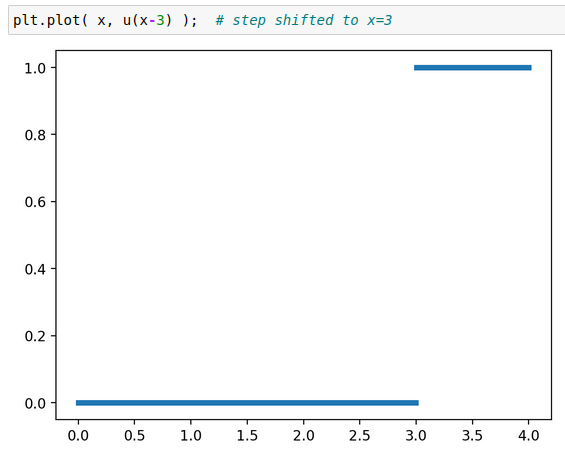
In order to use it, you'll need to come up with formulas for such forcing in terms of the Heaviside step function. We'll call it "u", and u(x) is 0 for x < 0 and 1 for x ≥ 0.
See if you can obtain formulas in terms of u for the following functions which have discontinuities and/or breaks in their slope.
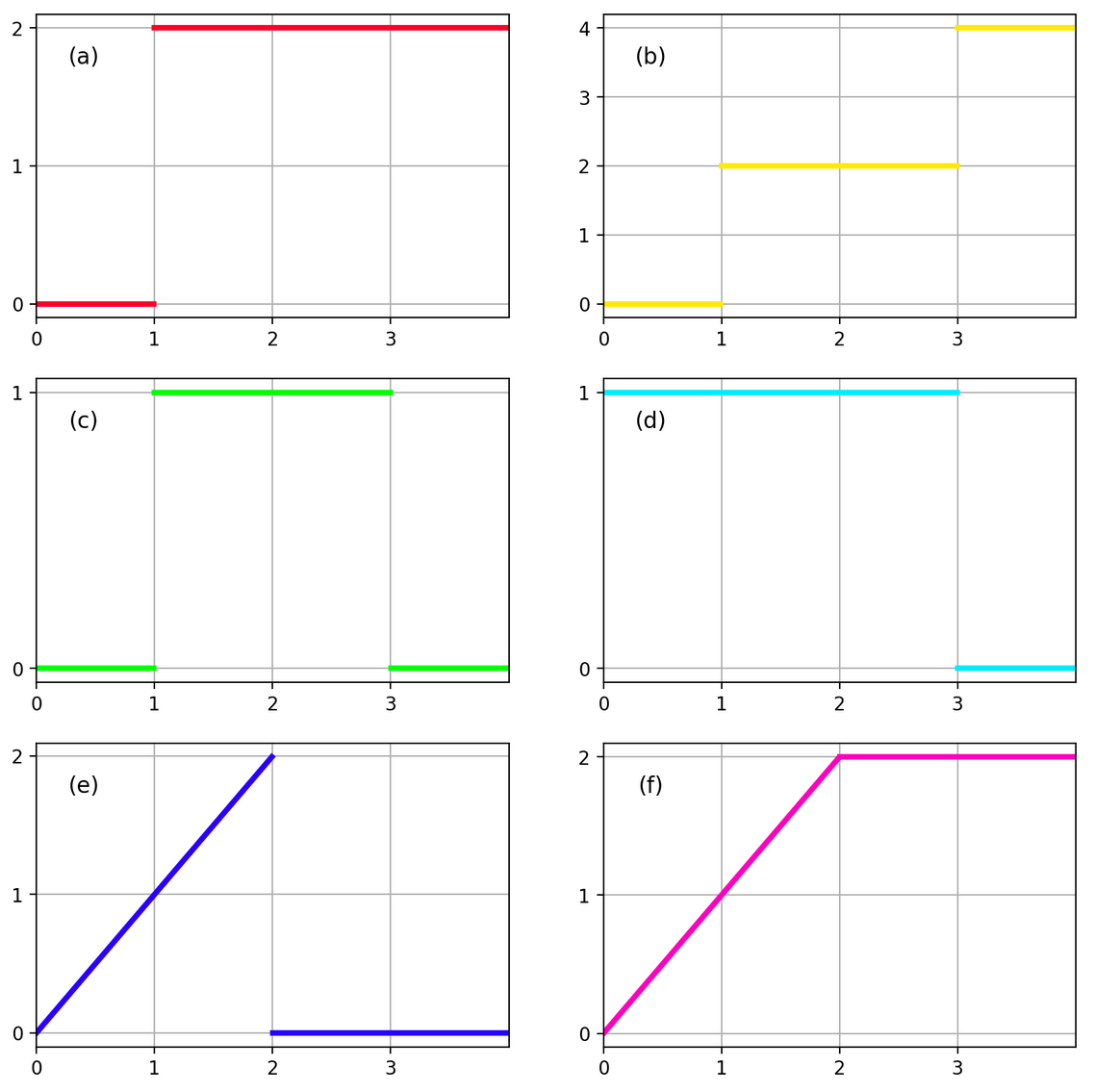
It's best if you can do this just by thinking with pencil and paper, but if you'd like to check your formulas, you can use this code to plot your formulas:
from resources306 import *
%config InlineBackend.figure_format = 'retina'
def heaviside(x):
         y = 0.5 * (np.sign(x) + 1)
         y[:-1][np.diff(y) >= 0.5] = np.nan  # break the line where the jump is
         return y
u = heaviside  # shorthand
x = np.linspace(0,4,1000)  # assume we're interested in x between 0 and 4
which you can use as follows: