Python utilities and demos for MTH 306
Contents
- Plotting a function
- Plotting solutions from formulas
- Slope field plot
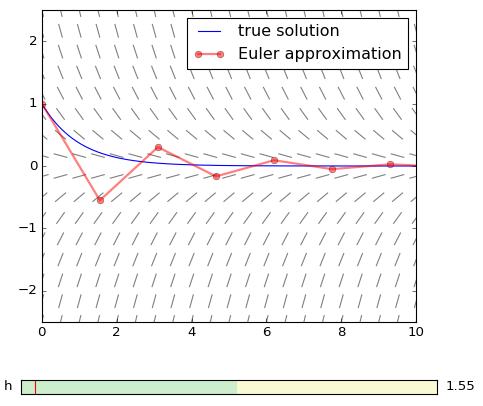
- Euler method instability
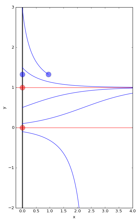
- Phase line animation and solution graph
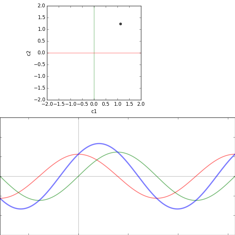
- Superposition of cos and sin with sliders and with a handle in the c1,c2-plane
- Solution by method of undetermined parameters
- Check solution of inhomogeneous 2nd order linear equation
- Forcing and resonance
- Solving DEs with sympy's dsolve
- Vector field plot
- Phase plane drawing
- 2D Euler with vector field
- Phase portrait for 2D linear system
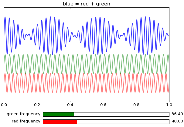
- Beats
- Lab 4 fishing animation
- Comparing nonlinear vector field and its linearization
- Power series solutions
- Laplace transform
Plotting a function
Here is how to plot a function or a family of functions.
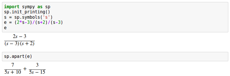
Plotting solutions from formulas
from numpy import *
from pylab import plot,show,xlim,ylim,savefig
def x(t,x0): return 13./(1-(1-13./x0)*exp(91*t))
t = linspace(0,0.02,100)
for x0 in linspace(0,15,16):
        plot( t, x(t,x0) )
xlim(0,.02)
ylim(0,20)
savefig('mysolutions.png')
show()
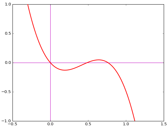
Another example, where the solutions involve a cube root:
Superposition of cos and sin with sliders and with a handle in the c1,c2-plane
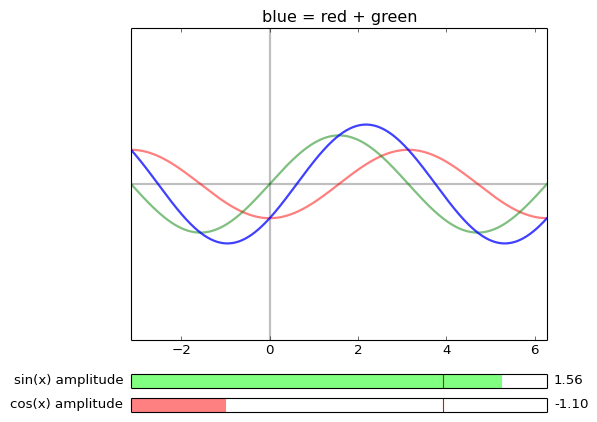
sin_plus_cos.py (drag the dot)
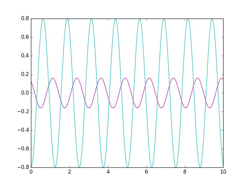
Solution by method of undetermined parameters
A second order linear equation solved analytically.
import sys
from sympy import *
t,a,b = symbols('t a b')

x = a*cos(5*t) + b*sin(5*t)

de =     x.diff(t,t) + 3*x.diff(t) + 5*x + 4*cos(5*t)    # style 1
de = Eq( x.diff(t,t) + 3*x.diff(t) + 5*x, -4*cos(5*t) )  # style 2 (both work)

de1 = de.subs(t,0)
de2 = de.subs(t,pi/10)

solution = solve( [de1,de2], [a,b] )
print( solution )
print( x.subs(solution) )
print( de.rhs )

from numpy import *
from pylab import plot,show,savefig
c1 = lambdify( t, x.subs(solution), 'numpy')
c2 = lambdify( t, de.rhs/5        , 'numpy')
t = linspace( 0., 10., 400 )
plot( t, c1(t), 'm', t, c2(t), 'c' )
savefig(sys.argv[0]+'.png')
show()
{a: 16/125, b: -12/125}
-12*sin(5*t)/125 + 16*cos(5*t)/125
-4*cos(5*t)
Check solution of inhomogeneous 2nd order linear equation
import sys
from sympy import *

alpha = atan2(18,-10)
print( alpha )

t = symbols('t')
x = sqrt(10**2 + 18*82)*cos(5*t - alpha) + 10*cos(4*t)
print( x )

lhs = simplify( diff(x,t,t) + 25*x )
rhs = simplify( 90*cos(4*t) )
print( lhs )
print( rhs )
print( lhs == rhs )

xf = lambdify(t,x,'numpy')
from numpy import *
import pylab as plt
plt.figure(figsize=(12,4),facecolor='white')
t = linspace(0,20,2000)
plt.plot( t, xf(t), lw=1.5, alpha=0.8)
plt.savefig(sys.argv[0]+'.svg')
plt.show()
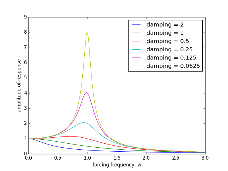
Forcing and resonance
# forced_damped_oscillator.py

from sympy import *
a  = symbols('a')
b  = symbols('b')
w  = symbols('w')
w0 = symbols('w0')
p  = symbols('p')
t  = symbols('t')
G0 = symbols('G0')

x = a*cos(w*t) + b*sin(w*t)
de = Eq(diff(x,t,t) + 2*p*diff(x,t) + w0**2*x, G0*cos(w*t) )
dec = de.subs(t,0)
des = de.subs(t,pi/2/w)
print(dec)
print(des)

sol = solve([dec,des],[a,b])
amp = simplify( sqrt(a**2 + b**2).subs(sol) )
print( amp )

amp = amp.subs({G0:1,w0:1})
from numpy import *
import pylab as plt
wvals = linspace(0,3,300)
for pval in [2,1,0.5,0.25,0.125,0.0625]:
        ampp = lambdify( w, amp.subs(p,pval), 'numpy' )
        plt.plot( wvals, ampp(wvals),label='damping = '+str(pval) )
plt.legend()
plt.xlabel('forcing frequency, w')
plt.ylabel('amplitude of response')
import sys
plt.savefig(sys.argv[0]+'.png')
plt.show()
-a*w**2 + a*w0**2 + 2*b*p*w == G0
-2*a*p*w - b*w**2 + b*w0**2 == 0
sqrt(G0**2/(4*p**2*w**2 + (w**2 - w0**2)**2))
Solving DEs with sympy's dsolve
Sympy has a command dsolve for solving differential equations. I don't want you to rely on it heavily in this course, because here we are trying to learn some of what goes on inside dsolve!
However, it is nice to have it available to check solutions that we have found by hand calculation, and in this section I'll show you how to do that.
Suppose we want to solve the initial value problem consisting of the following inhomogeneous linear 2nd order differential equation
y’’(x) + 2y’(x) + y(x) = sin2x
and the initial conditions
y(0) = 3,
y’(0) = 7.
Here's how you can do it. First we'll import sympy and start pretty printing:
from sympy import *
init_printing()
Then define the symbols we're going to use, and establish the DE. Note that to set up an equation we use the sympy function Eq and give it the RHS and LHS of the equation separated by a comma.
x = symbols('x')
y = symbols('y',cls=Function)
diffeq = Eq(y(x).diff(x, x) + 2*y(x).diff(x) + y(x), sin(2*x))
diffeq
Next we use dsolve to find a general solution formula:
sol = dsolve(diffeq)
sol
Wow! That was a lot easier than doing it by hand!
It remains to plug in the initial conditions and solve for the coefficients C1 and C2. To do this, I'll begin by pulling out just the right hand side of the expression dsolve gave us:
y = sol.rhs
y
Then I'll set up the two initial conditions:
ic1 = Eq( y.subs(x,0), 3 )
ic1
ic2 = Eq( diff(y,x).subs(x,0), 1 )
ic2
and use solve to solve the initial conditions for the coefficients C1 and C2:
coeffs = solve( [ic1, ic2] )
coeffs
Finally, I'll plug those values of the coefficients into the general solution formula:
y = y.subs(coeffs)
y
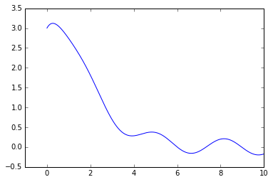
We can now plot the solution if we like:
from numpy import linspace
%matplotlib inline
import matplotlib.pyplot as plt
Y = lambdify(x,y,'numpy') # make a numpy-friendly function out of the solution expression
X = linspace(0,10,500)
plt.plot(X,Y(X))
plt.xlim(-1,10);
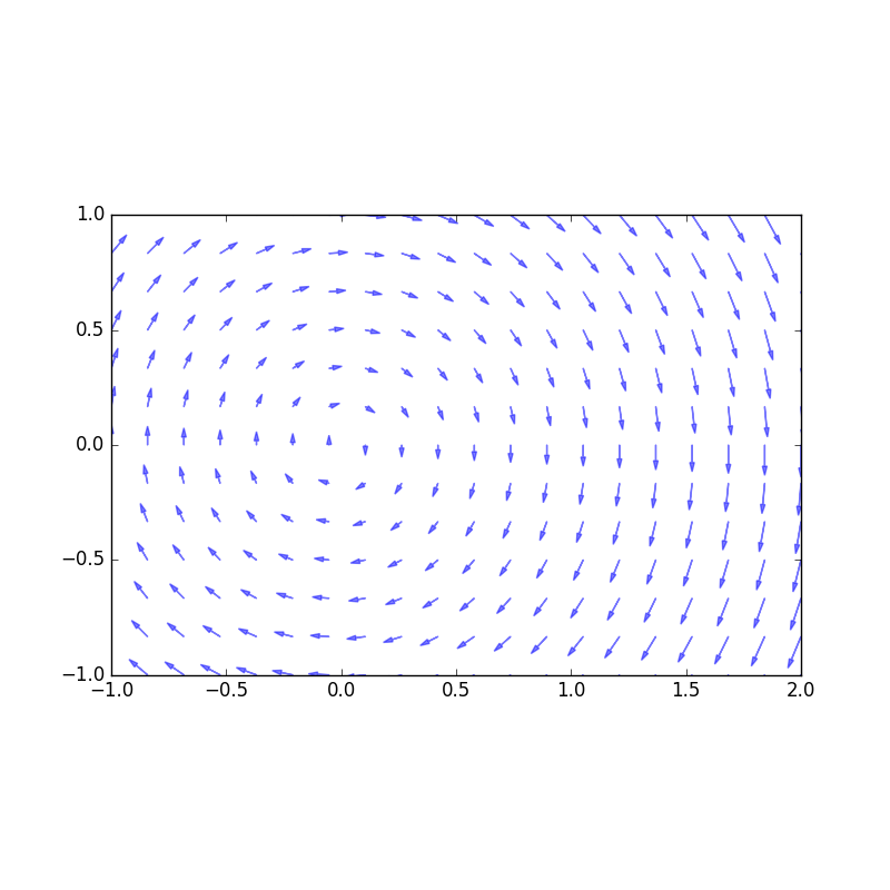
Vector field plot

from fieldplot import fieldplot
from pylab import show

def f(x,y): return  y
def g(x,y): return -x

fieldplot(f,g,-1,2,-1,1,aspect=1)

show()
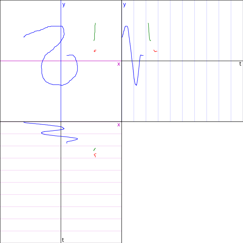
Phase plane drawing
User draws in xy-plane. Corresponding x vs t and y vs t graphs are drawn by the program.
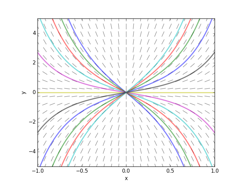
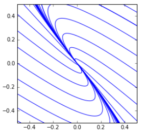
Phase portrait for 2D linear system
from sympy import *
init_printing()
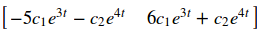
t,c1,c2 = symbols('t c1 c2')
mygensol = c1 * Matrix([[-5,6]]) * exp(3*t) + c2 * Matrix([[-1,1]]) * exp(4*t)
mygensol
def particularsol(gensol,t,t0,X0):
         gensolt0 = gensol.subs(t,t0)
         eq = Eq( gensolt0, X0 )
         c = solve( eq, [c1,c2])
         return gensol.subs(c)
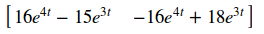
X0 = Matrix([[1,2]])
psol = particularsol(mygensol,t,0,X0)
psol
%matplotlib inline
from numpy import linspace, pi
import pylab as plt
plt.subplot(111,aspect=1)
t0 = 0.0
tmin = -2
tmax = 0
tt = linspace(tmin,tmax,200)
thetas = linspace(0,2*pi,50)
for theta in thetas:
         X0 = Matrix([[cos(theta),sin(theta)]])
         x,y = particularsol(mygensol,t,t0,X0)
         ux = lambdify(t,x,'numpy')
         uy = lambdify(t,y,'numpy')
         plt.plot(ux(tt),uy(tt),'b')
plt.xlim(-.5,.5)
plt.ylim(-.5,.5);
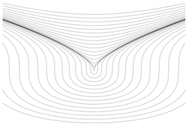
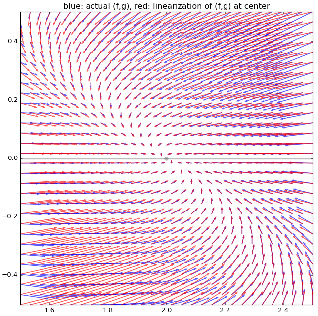
Comparing nonlinear vector field and its linearization
# nonlinear_vector_field_and_linearization.py

from sympy import symbols,diff
from fieldplot import fieldplot
import matplotlib.pyplot as plt

def f(x,y): return 2*x - x**2 -   x*y
def g(x,y): return 3*y - y**2 - 2*x*y

x0 = 2; y0 = 0; # center of plot and point we linearize at

x,y = symbols('x,y')
p0 = {x:x0,y:y0}

f0 = float(f(x,y).subs(p0))
g0 = float(g(x,y).subs(p0))

a = float(diff(f(x,y),x).subs(p0));  b = float(diff(f(x,y),y).subs(p0))
c = float(diff(g(x,y),x).subs(p0));  d = float(diff(g(x,y),y).subs(p0))

def lf(x,y): return f0 + a*(x-x0) + b*(y-y0)
def lg(x,y): return g0 + c*(x-x0) + d*(y-y0)

R = 0.5  # plot-window radius
plt.figure(facecolor='w')
plt.subplot(111,aspect=1)

plt.plot(x0,y0,'ko',alpha=0.25,markersize=7)
plt.plot([x0-R,x0+R],[0,0],'k',lw=3,alpha=0.25) # x-axis
plt.plot([0,0],[y0-R,y0+R],'k',lw=3,alpha=0.25) # y-axis
fieldplot( f, g,x0-R,x0+R,y0-R,y0+R,nx=30,color='b',boostarrows=5.)
fieldplot(lf,lg,x0-R,x0+R,y0-R,y0+R,nx=30,color='r',boostarrows=5.)

plt.title('blue: actual (f,g), red: linearization of (f,g) at center')
plt.show()
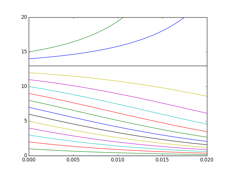
Power series solutions
Illustrating partial sums and radius of convergence
# taylor_series_solution_convergence.py
from numpy import *
import pylab as plt
import sys
x = linspace(-2,2,1000)
nmax = 40
c0 = 1
c1 = -1
terms = array(
              [c0*(-1)**n*x**(2*n  )/2**n +
               c1*(-1)**n*x**(2*n+1)/2**n for n in range(nmax+1)] )
psums = terms.cumsum(axis=0)
print(psums)
plt.plot(x,psums.T,alpha=0.25)
plt.ylim(-1,1.5)
plt.savefig(sys.argv[0]+'.png')
plt.show()

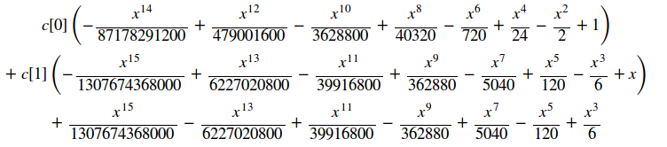
Computing coefficients
from sympy import *
init_printing()
def myde(x,y): return diff(y,x,x) + y - x
N = 15  # will solve for c[0] ... c[N]
x = symbols('x')
c = symbols('c[:' + str(N+1) + ']')  # for example, 'c[:7]'
y = sum( c[n]*x**n for n in range(N+1) )
de = Poly(expand( myde(x,y) ) , x)   # use Poly because it provides all_coeffs()
coeffs = de.all_coeffs()[::-1]       # reverse so that element n is of x**n
sol = solve(coeffs[:-2],c[2:N+1])
Y = collect(expand(y.subs(sol)),c)
Y
Laplace transform
from sympy import *
init_printing()
from sympy.integrals import laplace_transform, inverse_laplace_transform
Forward transform
s,t = symbols('s t')
w = symbols('w')
laplace_transform( sin(w*t), t, s )
# extract the part we want
laplace_transform(sin(w*t),t,s)[0]
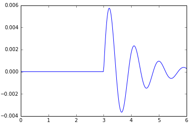
Inverse transform
F = exp(-3*(s+1))/((s+1)**2+49)
F
f = inverse_laplace_transform(F,s,t)
f
To make a ufunc out of this expression, we need to provide a translation for 'Heaviside', which does not exist in numpy
import numpy as np
def H(z): return 1.*(z>=0)
ff = lambdify(t,f,['numpy',{'Heaviside':H}])
tt = np.linspace(0,6,300)
%matplotlib inline
import pylab as plt
plt.plot(tt,ff(tt));
Doing the integral ourselves
# JR 6/23/14
# Assumptions need work and thinking about

from sympy import *

s,t = symbols('s t')

def L(y):
        var('s',positive=True)
        return integrate( y*exp(-s*t), (t, 0, oo) ).simplify()

a,b = symbols('a b')
var('a',positive=True)
var('b',positive=True)

for y in [1,t,t**2,sin(2*t),exp(-t)*sin(2*t),exp(-a*t)*sin(b*t)]:
        print( y, '\t', L(y) )
1       1/s
t       s**(-2)
t**2    2/s**3
sin(2*t)        2/(s**2 + 4)
exp(-t)*sin(2*t)        2/((s + 1)**2 + 4)
exp(-a*t)*sin(b*t)      b/(b**2 + (a + s)**2)