438/538 HW2 Solutions

Assignment 2
- 2.1
- 2.2
- 2.3
- 2.4
- 2.5

Assignment 2

Due in Room 244 Math Bldg, 3:29pm Friday, Feb 19.

2.1

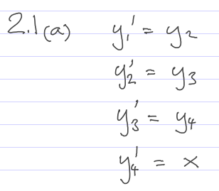
(a) 1pt Rewrite the fourth order equation y''''(x) = x as a 1st order system.

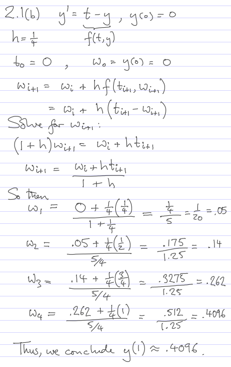
(b) 3pts By hand, solve the IVP y'=t-y, y(0)=0 for y(1) using 4 Backward-Euler steps (each of size h=1/4). Show all the steps of the calculation.

2.2

Euler and Backward Euler applied to xyz system with c=10000

This code, xyz_with_euler.py tries to solve the "xyz" system using Euler's method.

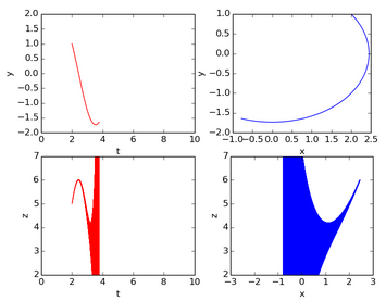
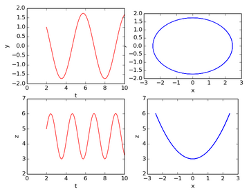
(a) 2pts Verify that Euler's method on this IVP is unstable with the number of steps n=49970, and stable with n=50030.

The two values of n give the results below: 49970 on the left, and 50030 on the right. On the left, z develops overshoots of unbounded amplitude (I broke out of the loop when |z| exceeded 20. On the right, with an ever-so-slightly smaller h, everything looks good: the solution seems quite accurate (no obvious spiraling out in the xy-plane).

(b) 2pts Compute the value of "ah" for this problem with the two different n-values, and relate your results in part (a) to our stability analysis of Euler's method. (Warning: the "a" in the stability analysis is not the "a" in parameters of this ODE.)

The "a" of our stability analysis is "-c" in the parameters of this ODE system. The values of ha are printed by the program,

print '"ha" =',  -h*c

and are -2.00120072043 for n=49970, and -1.99880071957 for n=50030. Our theoretical stability boundary is ha = -2, so these results are highly consistent with that!

(c) 5pts Modify the code to implement Backward Euler. Use scipy.optimize.fsolve to solve the implicit formula for w[i+1]. Verify that this method is stable, and also reasonably accurate, on this IVP with even as few steps as n=10000.

I just replaced "eulerstep" with the "backwardeulerstep" below:

def eulerstep(f,t,w,h,*args):
        return w + h*f(t,w,*args)

from scipy.optimize import fsolve

def backwardeulerstep(f,t,w,h,*args):
        def g(u): return -u + w + h*f(t,u,*args)
        u = fsolve( g, w )
        return u

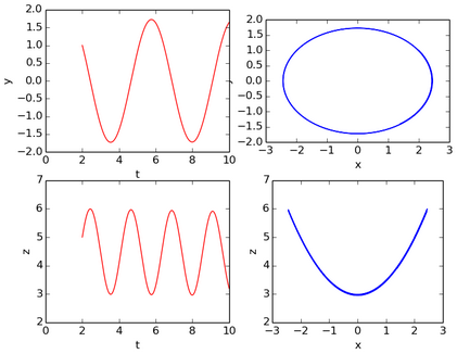
Even with n=10000 (5 times outside the Euler stability boundary), Backward Euler is stable:

(d) 1pt Why does z oscillate at twice the frequency that x and y do?

z is tracking x^2 + y^2, with (x,y) tracing an ellipse. So on a single circuit around the ellipse, x^2+y^2 goes from its maximum to its minimum (90 degrees later), back to its maximum (at 180 degrees), then back to its minimum, and finally back to its maximum as the circuit is completed. That's two full oscillations of x^2+y^2 for every oscillation of x or of y.

2.3

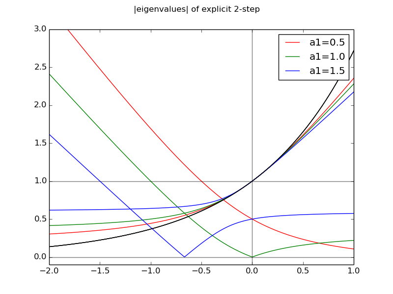
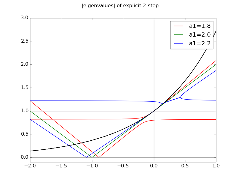
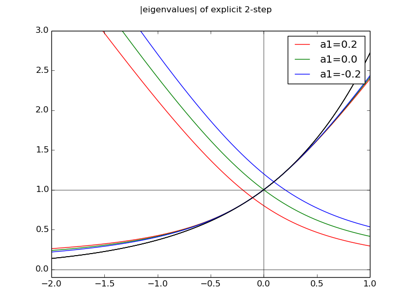
(a) (2pts) Take this code, multistep_stability.py, which plots, as a function of ha, the moduli ("magnitudes") of the eigenvalues for any explicit linear 2-step method of order 2 (local error O(h^3)), and try various values of the parameter, a1.

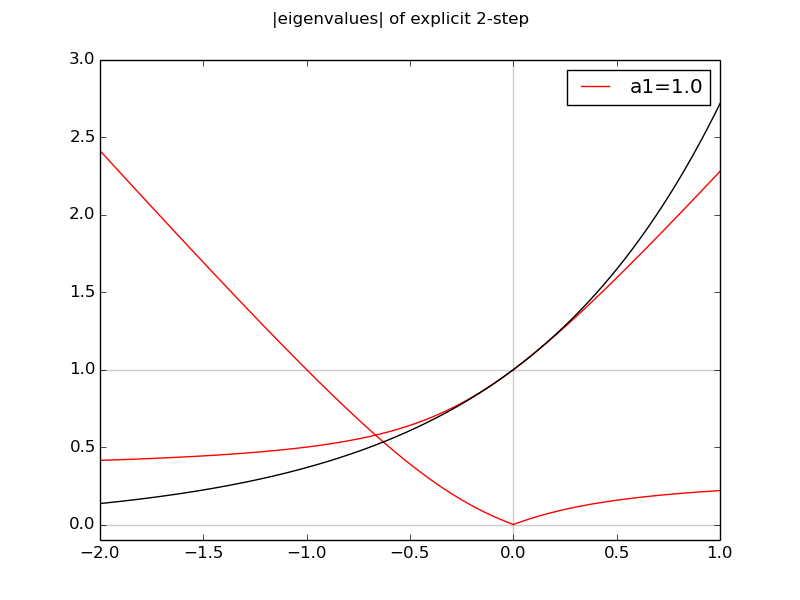
(b) (2pts) Discuss the differences seen in (a), and try to explain why only the choice a1=1 has a name! (I.e., Adams-Bashforth.) Note that the "correct" behavior on the linear model is shown in black in the plot.

First of all if we look at values not too far from the AB value of a1=1,

we see that there is a trade-off between accuracy and stability. It appears (and this can easily be verified algebraically) that the stability boundary is ha = a1. Thus increasing a1 from 1 enlarges the stability region, and decreasing a1 below 1 shrinks it. On the other hand, we can see by comparing how close the colored curve is to the black one, that the accuracy increases as a1 decreases.

Going to more extreme values of a1 ...

We see that for a1>2, (e.g. a1=3) there is an eigenvalue of modulus greater than 1 for all negative values of a1. That is, the method is unstable no matter what.

Going in the other direction, way below 1 ...

we see that for a1 positive but near 0, we have good accuracy, but a very narrow stability window (of width a1), and also a numerical mode that doesn't decay very fast, and for a1<=0, we have instability for all ah.

To summarize: The only usable values of a1 are 0 < a1 < 2. We have narrow stability region for a1 small, but the accuracy increases as a1 decreases. In this sense, Adams-Bashforth can evidently be considered a compromise between stability and accuracy.

2.4

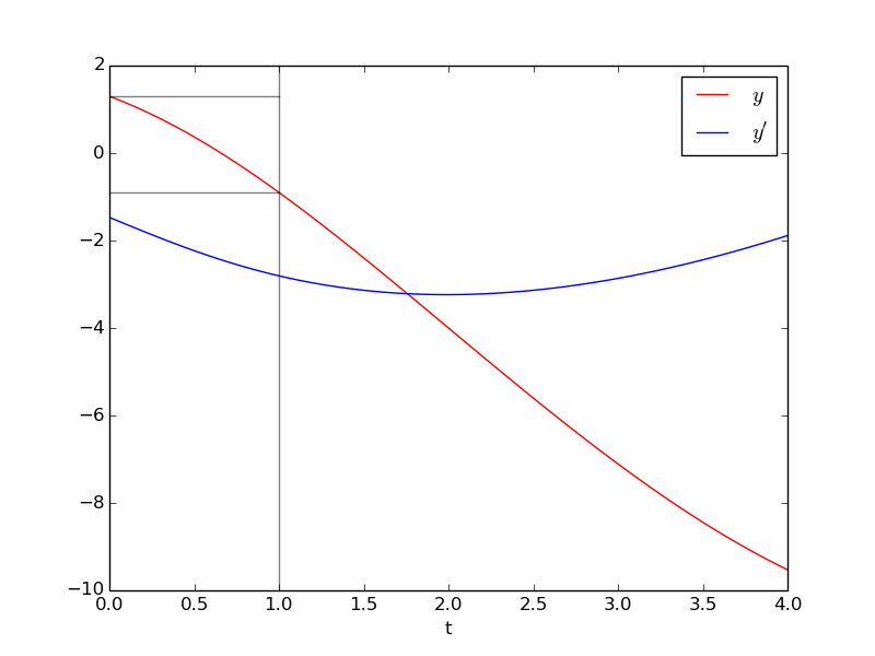
(6pts) Solve the BVP

y^′′(t) = (2t)/(1 + t²)y^′(t) − (2)/(1 + t²)y(t) + 1,

y(0) = 1.3,

y(1) = − 0.95

over the t-interval [0,4], by linear shooting (not by a general nonlinear iteration). Use the scipy.integrate.ode vode Adams IVP solver. Plot your solution (both y and y').

Here are my results. Final values are: 4.0 [-9.72752804 -1.93629735], fcount 158, jcount 4

from scipy.integrate import ode
import sys
from numpy import *
import matplotlib.pyplot as pl

def myf(t,yyp,homog=False):
      global fcount
      fcount += 1
      y,yp = yyp
      if homog:
              return array([ yp, (2.*t/(1.+t**2))*yp - (2./(1+t**2))*y       ])
      else:
              return array([ yp, (2.*t/(1.+t**2))*yp - (2./(1+t**2))*y + 1.  ])

def myjac(t,yyp):
      global jcount
      jcount += 1
      #y,yp = yyp
      return array([[ 0. , 1. ],
                  [ - (2./(1+t**2)), (2.*t/(1.+t**2)) ]] )

r = ode(myf, myjac).set_integrator('vode', method='adams',atol=1.e-10)

t1 = 1.

alpha =  1.3
beta  = -0.95

# first shot
r.set_initial_value([alpha,0.],0.)
fcount = 0
jcount = 0
y1,yp1 = r.integrate(t1)
t = r.t
print t,y1,yp1, fcount, jcount

# 2nd shot
r.set_initial_value([0.,1.],0.)
r.set_f_params(True)
y2,yp2 = r.integrate(t1)
t = r.t
print t,y2,yp2, fcount, jcount

c = (beta-y1)/y2
print c

# check, with dense output
n = 100
dt = 4./float(n)
data = empty((2,n+1))
data[:,0] = [alpha,c]
r.set_initial_value([alpha,c],0.)
r.set_f_params(False)
print r.integrate(1.)
r.set_initial_value([alpha,c],0.)
for i in range(n):
      if r.successful():
              data[:,i+1] = r.integrate((i+1)*dt)
      else:
              print 'r not successful', i*dt
              break

pl.plot( linspace(0,4,n+1), data[0,:], 'r', label='$y$')
pl.plot( linspace(0,4,n+1), data[1,:], 'b', label='$y^\prime$')
print r.t, data[:,-1], fcount, jcount

pl.plot([1,1],[-10,2],'k',alpha=0.5)
pl.plot([0,1],[alpha,alpha],'k',alpha=0.5)
pl.plot([0,1],[beta ,beta ],'k',alpha=0.5)
pl.legend()
pl.xlabel('t')
pl.show()

2.5

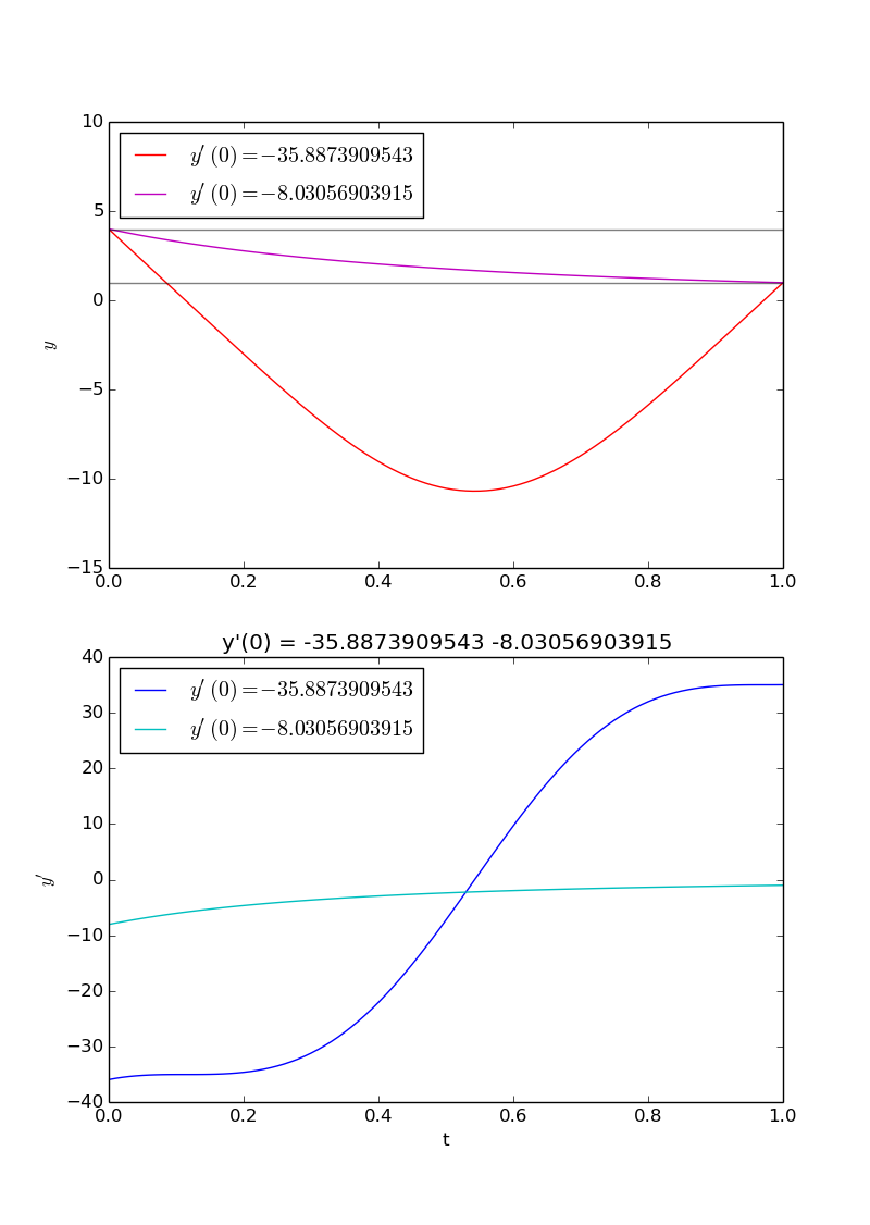
(6pts) Solve the (nonlinear) BVP

y^′′(t) = (3)/(2)y(t)²,

y(0) = 4.01

y(1) = 1

on the t-interval [0,1] by shooting. Use any accurate method you like for the IVP solving, and I recommend you use scipy.optimize.brentq to solve the boundary condition. Caution: there may be more than one solution of this BVP, so you may need to scan the IVP parameter to find them all. Plot your solution(s).

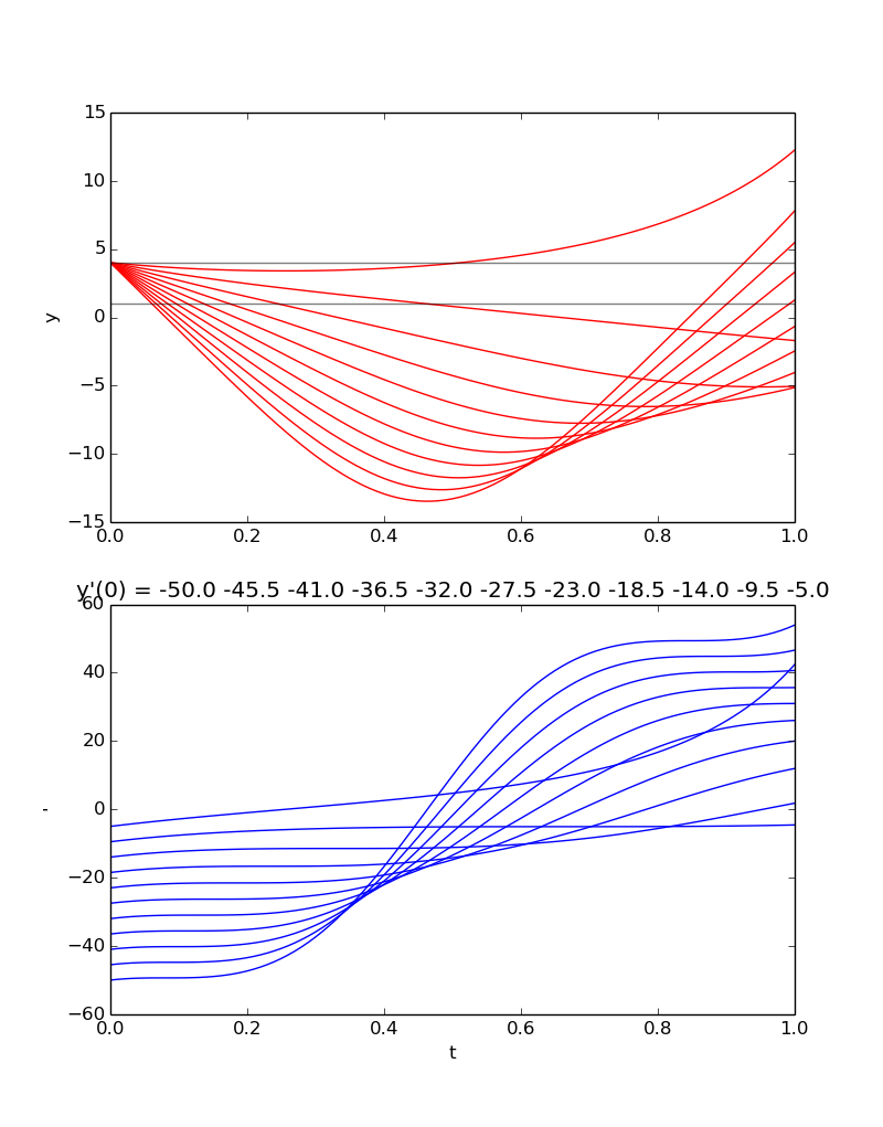
Initial scan of y'(0) ... well ok, after a bit of trial and error:

Looks like there are two solutions, based on these values for y(1):

 y'(0)         y(1)
-50.0 1.0 [  7.7988061   53.94341216] 100 2
-45.5 1.0 [  5.47938211  46.58661811] 196 4
-41.0 1.0 [  3.31243535  40.65608372] 288 5
-36.5 1.0 [  1.26943966  35.63473797] 388 7
-32.0 1.0 [ -0.66107601  30.97192949] 482 8
-27.5 1.0 [ -2.45894355  26.01775077] 575 9
-23.0 1.0 [ -4.03436313  19.97177019] 661 10
-18.5 1.0 [ -5.13048865  11.94703006] 745 11
-14.0 1.0 [-5.04371212  1.79217216] 810 12
-9.5 1.0 [-1.69388574 -4.57259925] 863 13
-5.0 1.0 [ 12.24636619  42.39281379] 940 14

One must lie for y'(0) between -36.5 and -32. And the other must lie between -9.5 and -5. Here is the code used for the above initial scan:

Now we can nail down the solutions using a root finder.

Here's the code that generated the plot above:

from scipy.integrate import ode
import sys
from numpy import *
import matplotlib.pyplot as pl
from scipy.optimize import brentq

def myf(t,yyp,homog=False):
      global fcount
      fcount += 1
      y,yp = yyp
      return array([ yp, 3.*y**2/2.       ])

def myjac(t,yyp):
      global jcount
      jcount += 1
      y,yp = yyp
      return array([[ 0.  , 1. ],
                  [ 3.*y, 0. ]] )

r = ode(myf, myjac).set_integrator('vode', method='adams',atol=1.e-10)
fcount = 0
jcount = 0

t1 = 1.

alpha =  4.01
beta  =  1.

def deviation(s):
      r.set_initial_value([alpha,s],0.)
      y,yp = r.integrate(t1)
      return y-beta

s1 = brentq(deviation,-36.5,-32.)
print s1

s2 = brentq(deviation,-9.5,-5.)
print s2

print fcount, jcount
svals = [s1,s2]
reds  = ['r','m']
blues = ['b','c']
n = 100
dt = t1/float(n)
data = empty((2,n+1))


for j,s in enumerate(svals):
      data[:,0] = [alpha,s]
      r.set_initial_value([alpha,s],0.)
      for i in range(n):
              data[:,i+1] = r.integrate((i+1)*dt)

      pl.subplot(211)
      pl.plot( linspace(0,t1,n+1), data[0,:], color=reds[j] , label='$y ^\prime (0)='+str(s)+'$')
      pl.subplot(212)
      pl.plot( linspace(0,t1,n+1), data[1,:], color=blues[j], label='$y ^\prime (0)='+str(s)+'$')
      print s, r.t, data[:,-1], fcount, jcount


pl.subplot(211)
pl.plot([1,1],[-10,10],'k',alpha=0.5)
pl.plot([0,1],[alpha,alpha],'k',alpha=0.5)
pl.plot([0,1],[beta ,beta ],'k',alpha=0.5)
pl.ylabel('$y$')
pl.legend(loc='upper left')
pl.subplot(212)
pl.xlabel('t')
pl.ylabel("$y^\prime$")
pl.title("y'(0) = "+' '.join(map(str,svals)))
pl.legend(loc='upper left')
pl.show()