Assignment 3 Solutions
Due in Room 244 Math Bldg, 3:29pm Friday, Feb 26.
3.1
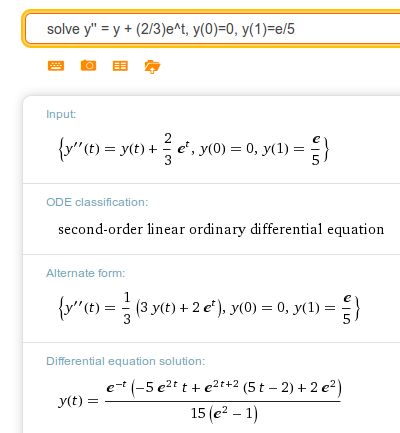
Consider the linear 2-point BVP on the t-interval [0,1]:
(a)(pts) Find a formula for the exact solution of this BVP.
(b)(pts) Write the finite difference approximation to the problem with 3 interior points, in matrix-vector form.
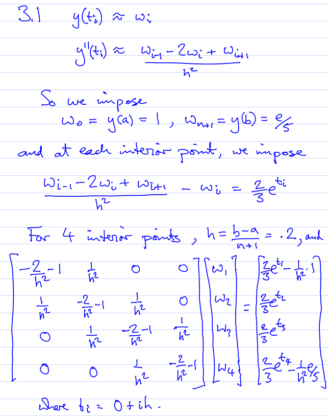
In the code for part (c) below, I multiplied the whole thing through by h^2.
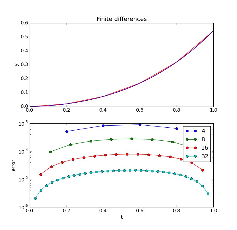
(c)(pts) Write a Python implementation of the finite difference method to solve this problem for n=4,8,16,32 interior points. Include code that makes plots of (i) the solution vs t, (ii) the |error| vs t, and (iii) |error| vs t on semilogy axes.
from numpy import *
def exact(t):
      return exp(-t)*( -5*exp(2*t)*t+ exp(2*t+2)*(5*t-2) + 2*exp(2) )/15/(exp(2)-1)
      from numpy import *
      from pylab import plot,show,ion,title,ylim,savefig,subplot,semilogy,legend,xlabel,ylabel
      import sys
from hw3exact import exact

      def prep_matrix(n):
              m = zeros((n,n))
              for i in range(n-1):
                      m[i,i+1]=1.
                      m[i+1,i]=1.
              return m

      a = 0.; ya = 0.
      b = 1.; yb = exp(1.)/5.
      gamma = 1.  # coefficient on RHS of ODE

      for n in [4,8,16,32]:
              m = prep_matrix(n)
              h = (b-a)/float(n+1)
              fill_diagonal(m,-gamma*h*h-2.)
              t = linspace(a,b,n+2)
              rhs = h**2*2./3.*exp(t[1:-1])
              rhs[ 0] -= ya
              rhs[-1] -= yb
              if n==4:
                      print 'matrix'
                      print m
                      print 'rhs'
                      print rhs
              y = linalg.solve(m,rhs)
              if n==4:
                      print 'solution'
                      print y

              t = linspace(a,b,n+2)
              subplot(211)
              plot( t,hstack(( [ya],y,[yb] )) ,'r' )
              subplot(212)
              semilogy( t,hstack(( [ya],y,[yb] )) - exact(t) ,'o-',label=str(n) )

      ylabel('error')
      xlabel('t')
      legend()
      subplot(211)
      ylabel('y')
      tt = linspace(a,b,500)
      plot( tt,exact(tt) ,'b' )
      title("Finite differences")
      show()
(d) Have your program print (i) the matrix, (ii) the right hand side, (iii) the solution, when h = (b-a)/5.
matrix
[[-2.04  1.    0.    0.  ]
 [ 1.   -2.04  1.    0.  ]
 [ 0.    1.   -2.04  1.  ]
 [ 0.    0.    1.   -2.04]]
rhs
[ 0.03257074  0.03978199  0.04858983 -0.48430861]
solution
[ 0.01984613  0.07305684  0.16897182  0.3202355 ]
3.2
Solve the same BVP as in 3.1 using the collocation method, the monomial basis, and the same set of numbers of points as in 3.1. Make the same plots you did in 3.1.
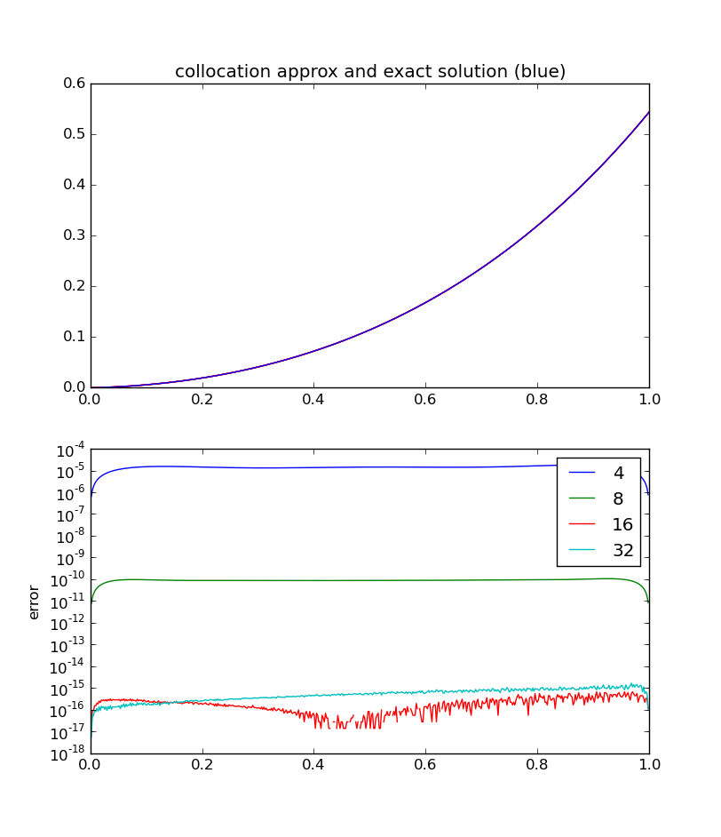
Note that the error is worse for n=32 than for n=16. This can be understood because the condition of the matrix is getting enormous as n increases:
n= 4 condition number of matrix 257.539990012
n= 8 condition number of matrix 691161.446079
n= 16 condition number of matrix 7.86930332029e+12
n= 32 condition number of matrix 6.19265152524e+18
We have to be careful about this! Perhaps we should consider using a different basis set.
      from numpy import *
      import pylab as pl
from hw3exact import exact

      def collocation_matrix(x,a,b,gamma):
              n = len(x)
              A = empty((n,n))

              for j in range(n): A[0  ,j] = a**j

              for i in range(1,n-1):
                      for j in range(n):
                              A[i,j] = float(j)*float(j-1)*x[i]**(j-2) - gamma*x[i]**j  # differs from chalk
                                                                                             # due to 0-based indexing
              for j in range(n): A[n-1,j] = b**j

              return A

      a = 0.; b = 1.
      alpha = 0.; beta = exp(1)/5.
      gamma = 1.

      for n in [4,8,16,32]:
              n += 2
              x = linspace(a,b,n)
              A = collocation_matrix(x,a,b,gamma)
              print 'n=',n-2,'condition number of matrix',linalg.cond(A)
              #print A
              rhs = 2./3.*exp(x)
              rhs[  0] = alpha
              rhs[n-1] = beta

              c = linalg.solve(A,rhs)
              #print c

              # evaluate our approximate solution on a dense grid
              xx = linspace(a,b,500)
              w = zeros_like(xx)
              for j in range(n):
                      w += c[j]*xx**j
              pl.subplot(211);
              pl.plot(xx,w,'r')
              pl.subplot(212); pl.ylabel('error')
              pl.semilogy(xx, abs(w-exact(xx)), label=str(n-2))  # error
      pl.legend()
      pl.subplot(211);
      pl.title('collocation approx and exact solution (blue)')
      pl.plot(xx,exact(xx),'b')

      pl.show()
(b) Have your program print (i) the matrix, (ii) the right hand side, (iii) the solution, when h = (b-a)/5.
n= 4 condition number of matrix 257.539990012
matrix
[[ 1.       0.       0.       0.       0.       0.     ]
 [-1.      -0.2      1.96     1.192    0.4784   0.15968]
 [-1.      -0.4      1.84     2.336    1.8944   1.26976]
 [-1.      -0.6      1.64     3.384    4.1904   4.24224]
 [-1.      -0.8      1.36     4.288    7.2704   9.91232]
 [ 1.       1.       1.       1.       1.       1.     ]]
rhs
[ 0.          0.81426851  0.9945498   1.21474587  1.48369395  0.54365637]
solution
[ 0.          0.02525275  0.33087512  0.12366176  0.04141806  0.02244868]
n= 8 condition number of matrix 691161.446081
n= 16 condition number of matrix 7.86924702595e+12
n= 32 condition number of matrix 1.77318210839e+19
3.3
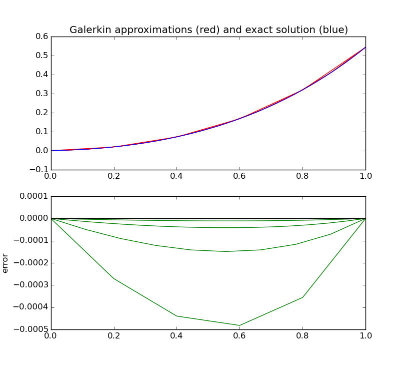
Solve the same BVP as in 3.2 using the Galerkin method, using the linear B-splines. Make the same plots you did in 3.2.
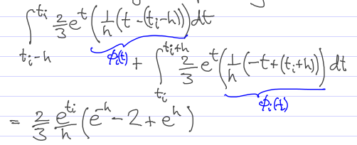
For this non-homogeneous equation, the RHS of the linear system we will solve for the {c_i} (which, because of the form of the linear B-splines, are themselves the approximations {w_i}) in all the rows except the first and the last is not zero, but rather the inner product of phi_i with the non-homogeneous term. Here is that integral:
And here is the max error vs h:
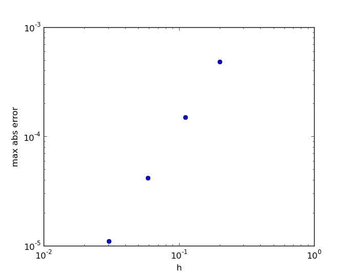
from numpy import *
import pylab as pl


def galerkin_matrix(t,gamma):  # for y'' = gamma y
        n = len(t)
        h = t[1]-t[0]
        print 'h',h
        A = zeros((n,n))
        A[ 0, 0] = 1.
        A[-1,-1] = 1.
        offdiag =  1./h -       gamma*h/6.
        diag    = -2./h - 2./3.*gamma*h
        for i in range(1,n-1):
                A[i,i-1] = offdiag
                A[i,i  ] = diag
                A[i,i+1] = offdiag
        return A

def galerkin_rhs_hw3(t,ya,yb):
        rhs = empty_like(t)
        h = t[1]-t[0]
        rhs[ 0] = ya
        rhs[-1] = yb
        rhs[1:-1] = 2./3.*exp(t[1:-1])/h*(exp(-h)-2.+exp(h))
        return rhs

a = 0.; b = 1.
alpha = 1.; beta = exp(1.)/5.
gamma = 1.

def exact(t):
        return exp(-t)*( -5*exp(2*t)*(t+3)+ exp(2*t+2)*(5*t-2) + 17*exp(2) )/15/(exp(2)-1)

errors = []
for n in [4,8,16,32]:
        n += 2
        t = linspace(a,b,n)
        A = galerkin_matrix(t,gamma)
        rhs = galerkin_rhs_hw3(t,alpha,beta)

        if n==6:
                print 'matrix'
                print A
                print 'rhs'
                print rhs
        c = linalg.solve(A,rhs)
        if n==6:
                print 'solution'
                print c

        pl.subplot(211); pl.title('n='+ str(n) + ' Galerkin approx (red) and exact solution (blue)')
        pl.plot(t,c,'r')
        pl.subplot(212); pl.ylabel('error')
        pl.plot(t, c-exact(t), 'g' )  # error
        pl.plot(t, 0*t, 'k' )

        errors.append( [n,abs(c-exact(t)).max()] )

pl.subplot(211);
pl.title('Galerkin approximations (red) and exact solution (blue)')
t = linspace(a,b,400)
pl.plot(t,exact(t),'b')


pl.figure(2); pl.xlabel('h'); pl.ylabel('max abs error')
pl.loglog([(b-a)/float(item[0]-1) for item in errors], [item[1] for item in errors], 'o')
pl.show()
(b) Have your program print (i) the matrix, (ii) the right hand side, (iii) the solution, when h = (b-a)/5.
h 0.2
matrix
[[  1.           0.           0.           0.           0.           0.        ]
 [  4.96666667 -10.13333333   4.96666667   0.           0.           0.        ]
 [  0.           4.96666667 -10.13333333   4.96666667   0.           0.        ]
 [  0.           0.           4.96666667 -10.13333333   4.96666667   0.        ]
 [  0.           0.           0.           4.96666667 -10.13333333
    4.96666667]
 [  0.           0.           0.           0.           0.           1.        ]]
rhs
[ 0.          0.16339727  0.19957388  0.24376008  0.29772924  0.54365637]
solution
[  8.38255639e-17   1.90627465e-02   7.17918999e-02   1.67594662e-01
   3.19225414e-01   5.43656366e-01]