Assignment 7
Due at the beginning of class, Tuesday, April 12.
Contents
7.1 DFT of audio clip
Obtain a short audio clip (a few seconds) of anything you like. Read it into a numpy array and compute the modulus of the DFT of the audio signal and plot it vs frequency in Hz. Comment on the features of the "spectrum" of your clip and relate them to what you hear when you listen to the sound. Note that there are free tools (especially for Linux) to convert among audio formats (wav, mp3, flac, ogg, etc.).
Compute and plot the DFT
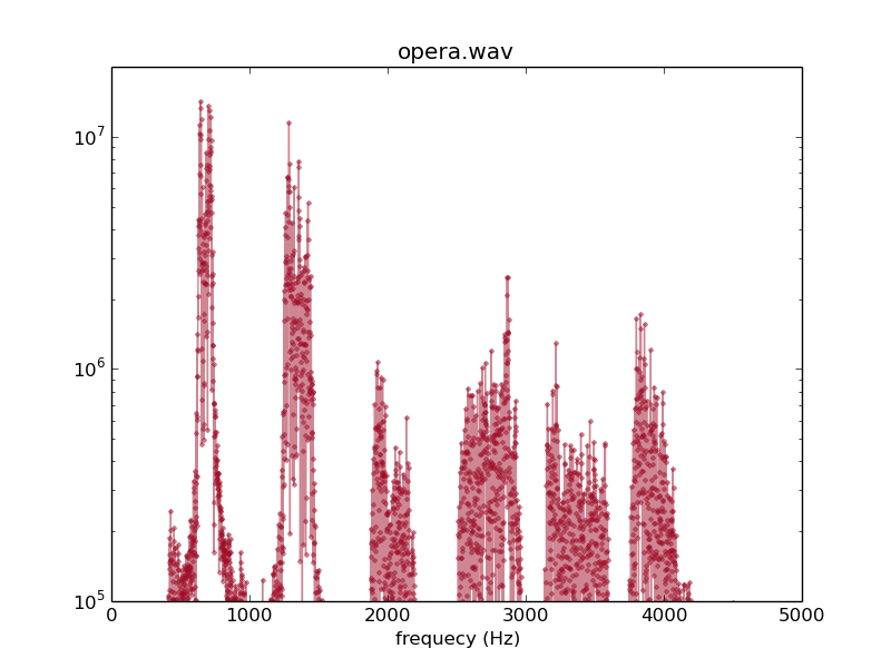
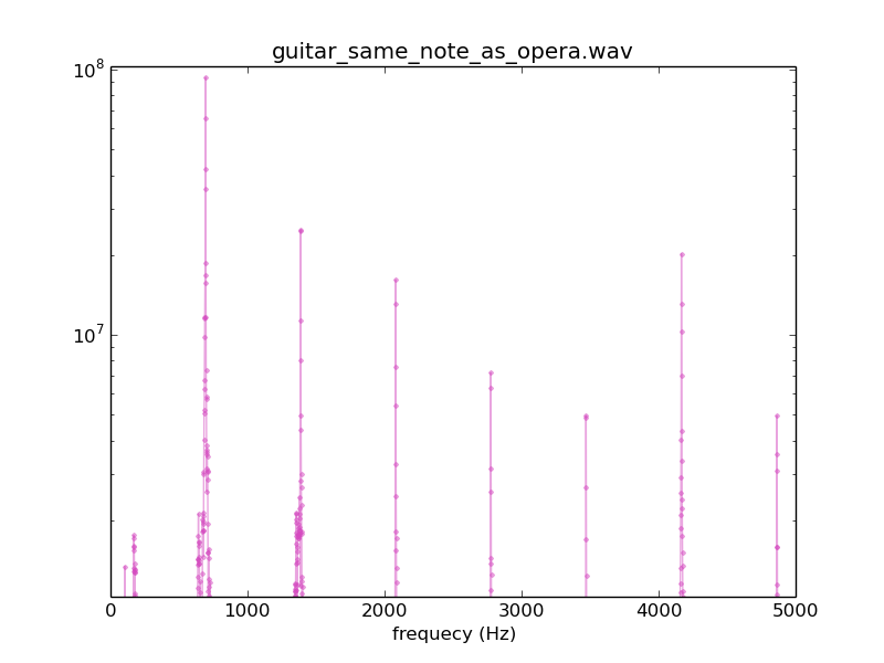
I will chose a 1-second long snippet of an opera singer with heavy vibrato (grabbed from Youtube), and compare its spectrum with that of a 1-second clip of a guitar note at approximately the same pitch.
Correspondence between spectrum and perceived sound
The gross features of the two pictures are the same: we see strong peaks at a "fundamental" (lowest) frequency, and at approximately integer multiples of it. However the peaks for the opera singer are much broader than those for the guitar which are extremely sharp. This is because the opera singer oscillates her pitch over quite a large range several times during the course of the sound clip.
The code used to make the pictures above is here:
# hw7.1fftaudio.py

from scipy.io import wavfile
from numpy import *
from randomhexcolor import randomhexcolor
wavfilename = 'guitar_same_note_as_opera.wav' #'opera.wav'
rate,x = wavfile.read(wavfilename)
print 'rate',rate
print 'x.shape',x.shape

n = x.shape[0]
d = n/float(rate)  # duration of recording
print 'duration',d,'secs'

import matplotlib.pyplot as plt
#plt.plot(x)
#plt.show()

from scipy.fftpack import fft

#print y
nchunks = 1 #80
m = n/nchunks
for i in range(nchunks):
        #plt.subplot(nchunks,1,i+1)
        if len(x.shape)>1: xchunk = x[i*m:(i+1)*m,0]
        else:              xchunk = x[i*m:(i+1)*m]
        y = fft(xchunk)
        print len(y), abs(y).max()
        #print i, argmax(y[:14])/float(d)*float(nchunks), 'Hz'
        plt.clf()
        plt.semilogy( arange(m)/(d/nchunks) , abs(y),'.-',markersize=5,alpha=0.5,color=randomhexcolor())
        #plt.xlim(0,4000)
        #plt.ylim(1e3,2e7)
        plt.xlim(0,5000)
        plt.ylim(abs(y).max()*1.1/100,abs(y).max()*1.1)
        plt.title(wavfilename)
        plt.xlabel('frequecy (Hz)')

        plt.savefig(wavfilename + '_' + str(i).zfill(3) + '.png')
#print type(x)

#plt.xlim(0,3000/d)
plt.show()
7.2 Inverse DFT: synthesis of a piano note
a Locate the peaks of the spectrum
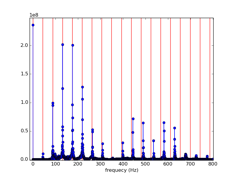
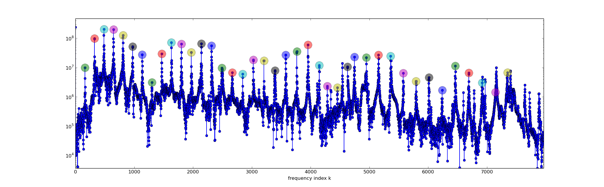
Determine the location (k-value) and height of the ~17 peaks of the spectrum of the piano low F that we computed in class on March 29 and that are visible in this plot.
This is not trivial. In principal we can characterize a maximum point as an index k where |yk − 1| < |yk| and also |yk + 1| < |yk|. But the vector y is "noisy" with lots of ups and downs, so this criterion (alone) will give us many spurious maximum points. Perhaps we can restrict our attention to windows around the integer multiples of the fundamental and use the location of the maximum of each of those subsets of the data. Thanks to Jackson for this idea!
from scipy.io import wavfile
from numpy import *
from scipy.fftpack import fft,ifft

rate,x = wavfile.read('piano_low_f.wav')
print 'rate',rate
print 'x.shape',x.shape

xmax = max(abs(x))
n = x.shape[0]
d = n/float(rate)  # duration of recording
print 'duration',d,'secs'

import matplotlib.pyplot as plt

y = fft(x)
a = abs(y)
plot = plt.semilogy
plot( arange(n), a, 'o-' )

###### try to find the maximum points ##############################

k0 = 161 #location of fundamental peak visually determined from plot
k  = k0
npeaks = 40  # number of peaks to capture (I did more than 17)
dk = 70  # half-width of window we'll take the max over
peaks = []

for ipeak in range(npeaks):
        kpeak = k-dk+a[k-dk:k+dk].argmax()
        peak = a[kpeak]
        peaks.append((kpeak,peak))
        print ipeak, kpeak, peak
        plot(kpeak,peak,'o',markersize=20,alpha=0.5)
        k = kpeak + k0
######## ###########################################################


plt.xlim(0,8000)
plt.xlabel('frequency index k')
plt.show()
It works pretty well, as you can see in the following plot where I've highlighted the peaks I found. There are some anharmonic peaks that I've missed, and these derail the algorithm at the high frequency end. Hopefully those very high frequency peaks are not essential.
b Make a caricature of the spectrum and generate a synthetic note
Construct a numpy array y that is all zeros except for real values equal to the 17 peak moduli at the corresponding indices, and also at the mirror image indices to make yn − k = yk for k = 1, 2, 3, ..., n − 1. Obtain the inverse DFT of your vector y, and save it as a wav audio file.
# synthesize piano sound from just the peaks
sy = zeros_like(y)
for kpeak,peak in peaks:
        sy[kpeak]   = peak
        sy[n-kpeak] = peak
newx = ifft(sy)
newx /= abs(newx).max()
#newx *= xmax
#newx /= 10
# Some trial and error done here:
# wavfile.write seems to expect the data to be between -1 and +1.
print newx
print 'xmax',xmax
print 'x data type',type(x[0])

intnewx = array( real(newx), dtype=int16 )
print 'intnewx.max()',abs(intnewx).max()

wavfile.write('synthesized_piano.wav',rate,real(newx))
c Reflection
Comment on the similarity or otherwise of this synthesized sound and the original piano
Here is the resulting wav file. To my ear, it sounds very similar to the original piano note. The main difference is that the characteristic percussive start of the original piano recording is not there, and most notably, the amplitude does not decay over the course of the synthesized clip.
Note: I think this clearly demonstrates that the phase of the frequency components is not detectable by our ears - if the above synthesis we set all the phases to "0" by making all the components of y real.
7.3 Symmetry of DFT of real vector
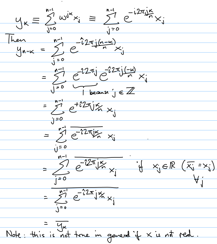
Prove that if x is in R^n (i.e. x is a real n-vector), then its DFT y satisfies yn − k = yk for k = 1, 2, 3, ..., n − 1. Hint: Sauer textbook.
In the proof below, I use the facts that the conjugate of a product is the product of the conjugates and likewise for a sum.