1.

[4 points]

Take the last 4 digits of your UB person number, interpreted as a decimal integer, and divide by 100. By hand, determine the binary representation the resulting number. (For example, if your person number were 87654719, you'd find the binary representation of 47.19.) Use the repeated multiplying and dividing by 2 method shown in class, and show all your work.

2.

A floating point system similar to the IEEE 754 system has: a sign bit, then a 2-bit exponent biased by 2, then a 3-bit mantissa. Assuming all bit-codes are used for numbers, and that the all-zeros code is used for 0 ...

a [4 points] List all the non-negative machine numbers in this system if denormalization is NOT used. For each, give the bit-code in both binary and hex form (pad with zeros on the left for the hex conversion), the number it represents - in binary fixed-point form (e.g. 110.0101), and finally in decimal notation (e.g. 1.875).

b What is the smallest positive machine number with and without denormalization. For each, give all the forms requested in part a.

c [1 point] The "machine epsilon" or εmach, defined to be the difference between 1 and the next larger machine number, is a very important characteristic of a floating point number system like this. What is εmach for this system?

d [1 point] How big is the "hole at zero" for this system in part (a), i.e. the gap between the smallest positive number and 0?

e [1 point] How big is the hole at zero in part (b)?

f [1 point] What would be the largest number in the system if the top exponent code were reserved for "Inf"s and "NaN"?

Note to self: The now-reduced part b can be omitted because it's covered in part d.

3.

[5 points] Derive by hand the hexadecimal machine IEEE 754 64-bit code for the number 9.3. Show all the steps clearly.

1.

Consider the difficulty of accurately evaluating sin x - x when x is near 0.

a [5 points] Find an approximate bound for the relative rounding error in evaluating the formula directly (in terms of machine epsilon). The desired answer is a small multiple of machine epsilon divided by a power of x. You may use low-order Taylor polynomial approximations and discard higher order terms when appropriate in order to get this answer.

b [3 points] Find a bound on the relative truncation error incurred by using the approximation sin x - x ~ -x^3/3! + x^5/5! - x^7/7!.

c [5 points] If we use the approximation sin x - x ~ -x^3/3! + x^5/5! - x^7/7!, for approximately which values of x (near 0) will the approximation be evaluated more accurately than the formula sin x - x itself if we are using arithmetic with machine epsilon = 2^-52? How many decimal digits are reliable in the worst case if we use the approximation and direct evaluation in the appropriate ranges? It is essential that you show all your work and make your reasoning clear to the grader!

2.

a Ackleh 2.10.1(a) [3 points]

b Ackleh 2.10.3 using Python. [(a) 3 points, (b) 3 points]

c Ackleh 2.10.4 (4th root of 1000) [1 point]

Python formatting hint (uses an "f-string"):

print(f'{1/300:+.8f} {1/300:.15e} and {777:4d}')

+0.00333333 3.333333333333334e-03 and  777

1.

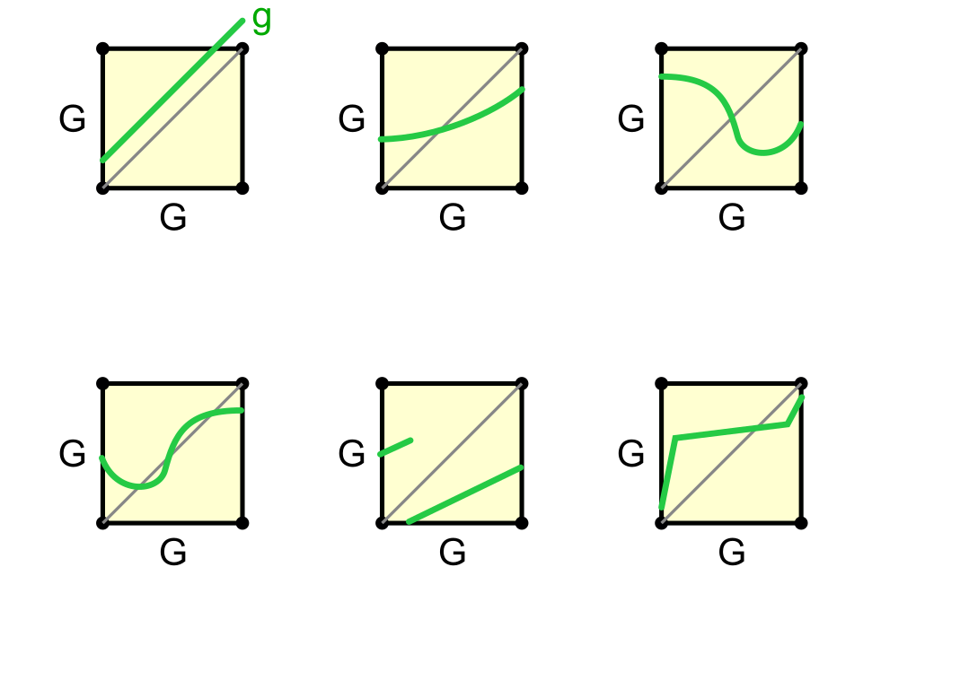
For each of the 6 functions, g, whose graphs are sketched below:

• If g does not have a unique fixed point in G, state a hypothesis of the Contraction Mapping Theorem that is not satisfied by g.
• If g does have a unique fixed point in G but iteration of g (starting in G) does not certainly converge to that fixed point, state a hypothesis of the CM theorem that is not satisfied by g.
• If g is not a contraction, mark 2 points x, y such that |g(x) − g(y)| ≥ |x − y|
• If g is does not map G into G, mark a point p in G such that g(p) is not in G.
• If iteration of g converges to a unique fixed point despite g not satisfying the hypotheses of the CM Theorem, circle the picture.

2.

Consider the example g(x) = (x² + 6) ⁄ 5 on G=[1,2.3]. Show that g maps G into G and show that g is a contraction, either by brute force or using appropriate Propositions from Section 2.3.

3.

Transcribe the statement and proof of Proposition 2.3, p 42, explain the hypothesis that's in addition to g being a contraction, and explain and/or justify each step of the proof.

1.

Prove that for a real nxn matrix, the matrix norm induced by the vector infinity-norm is the maximum row sum of absolute values.

2.

The following code generates 2000 random linear systems and a random perturbation of each, and makes a picture. Run it and describe/show how the results are consistent or not with Theorem 3.10.

import numpy as np
import matplotlib.pyplot as plt

def vnorm(x): return np.abs( x ).max()   # alternatively np.linalg.norm(x,np.inf)
def mnorm(a): return np.abs(a   ).sum(axis=1).max()

n = 5

plt.subplot(111,aspect=1)

for k in range(2000):

         a0 = np.random.randn(n,n)  # random base matrix
         a0inv = np.linalg.inv(a0)
         ka = mnorm(a0)*mnorm(a0inv)

         x0 = np.random.randn(n)        # solution of base system
         b0 = a0@x0                # right hand side of base system

         delta = 1.e-6*np.random.rand()   # random magnitude of perturbation
         da = delta*np.random.randn(n,n)  # random perturbation of matrix
         db = delta*np.random.randn(n)    # random perturbation of right hand side
         a = a0 + da
         b = b0 + db

         x = np.linalg.solve(a,b)  # solve perturbed system using GEPP
         dx = x - x0

         lhs = vnorm(dx)/vnorm(x0)  # relative change in solution
         rhs = float( ka/(1 - mnorm(da)*mnorm(a0inv))*( vnorm(db)/vnorm(b) + mnorm(da)/mnorm(a) ))  # bound on relative change from Theorem 3.10

         plt.loglog(rhs,lhs,'o',ms=1,alpha=0.5)

plt.xlabel('RHS')
plt.ylabel('LHS');

3.

Perform GE(PP) by hand on the matrix

[ 1  0  0  0  1 ]
[-1  1  0  0  1 ]
[-1 -1  1  0  1 ]
[-1 -1 -1  1  1 ]
[-1 -1 -1 -1  1 ]

demonstrating that the bound 2^n − 1 on the growth rate in GEPP can in fact occur. Show the intermediate result just for each "k", not for every single row operation.

4.

The Hilbert matrices are a classic example of ill-conditioned matrices. As you know, the condition number of a matrix in any norm is the product if the norms of the matrix and of its inverse.

Although accurately computing the inverse of an ill-conditioned matrix is problematic in general, the Hilbert matrices have rational elements, hence so do their inverses, and since sympy can do rational arithmetic exactly, we can compute the inverses of the Hilbert matrices exactly. Here is code to construct the Hilbert matrices and their inverses with sympy:

# sympy for exact inverse of Hilbert matrix
import sympy as sp
# construct the Hilbert matrix of order n
a = sp.ones(n)
for i in range(n):
         for j in range(n):
             a[i,j] /= (1+i+j)
display(a)
ainv = a.inv()
ainv

and here is a way to compute the infinity norm (maximum row sum of absolute values) of a matrix using numpy (which has a nicer operation set than sympy):

np.abs(m).sum(axis=1).max()

(Numpy can handle m being a sympy Matrix.) Make sure you understand how the above line of code works.

1. Compute H^− 1₅ exactly.
2. For n ranging from 1 to 10, compute exactly: the infinity norms of H_n and H^− 1_n, the (infinity-norm) condition number of H_n in scientific notation (like 4 × 10⁹, so I can see at a glance how big it is).

(c) For each value of n from 1 to 10, construct and use numpy.linalg.solve() (GEPP) to solve 4000 randomly chosen linear systems H_nx = b and compute the largest relative error in your solutions and the error bound provided by Wilkinson's theorem assuming the worst possible growth rate, ρ. (n on the horizontal axis, log error on vertical; a dot for the worst error in your 4000 trials, and a dot for the Wilkinson error bound.) Comment on the results.

1.

2.

In solving a linear system Ax=b with finite-precision arithmetic, we have a (Wilkinson) bound on the norm of error relative to the solution: ||error|| ⁄ ||x||. For example, in Homework 4, Question 4, I found that the relative error bound with ϵ_mach = 2^− 52 for systems with Hilbert matrix H₃ is about 2 × 10^− 11.

This does not mean that each component of the solution has this relative accuracy.

Provide an example of a pair of 3-vectors x and an approximation x̃, for which the norm of the difference relative to the norm of x is 1% while there is a 100% error in one of the components.

3.

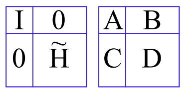
1. What is the product of the following block matrices? I is an identity matrix.

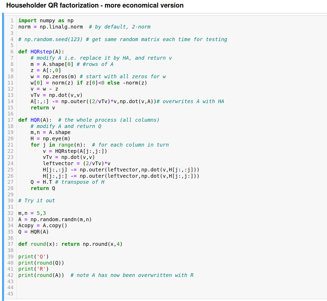
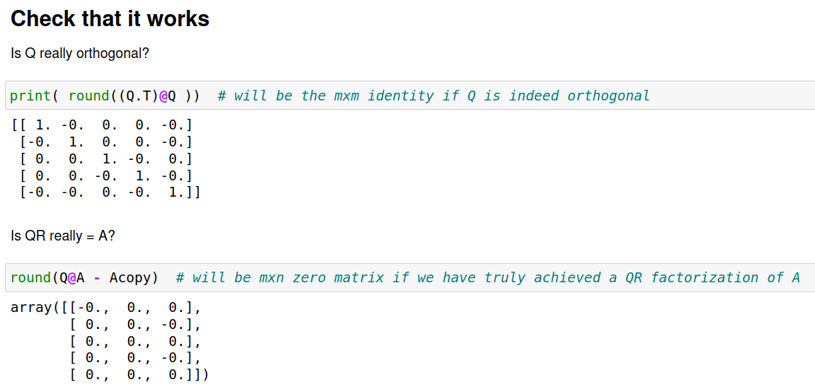
(b) Below I have written a version of Householder QR that is more economical than the one I wrote in class by avoiding matrix-matrix multiplication to form each H_i in HQRstep. Obtain an exact count of the number of arithmetic operations used by this implementation of HQR applied to an mxn matrix with m ≥ n. Begin by obtaining a formula (you can use sympy to do the sum) for the operation count for HQRstep applied to an MxN matrix. (M,N will start as m,n and be succcesively smaller by 1 at each stage.)

Include in your answer the code annotated with the operation cost for each line.

Note that this is still not the optimal implementation of Householder QR, which would avoid ever forming Q, and simply provide the list of v's that determine Q.

1. Example of polynomial interpolation

a Write down in Lagrange form, without simplifying, a polynomial that passes through the points (0,3), (2,3), (3,5), (6,4).

b Simplify by cleaning up the numerical coefficients, but do not multiply out the (x-x_i) terms.

c Re-express the polynomial in the monomial basis by expanding products and collecting terms.

d Plot the polynomial on the interval [0,6] and add dots at the data points.

e Modify the code we wrote in class on Day 13 to use the Newton basis instead of the monomial basis, and graphically verify the generated polynomial is the same. Suggestion make the first curve dark-colored and thick (say linewidth=3) and the second one light-colored and thin.

2. Error bound for interpolating polynomial

Prove Thm 4.6. Please take only one logical step per line, and justify every step to the extent needed to make it clear to yourself. At the end, state which step required the most ingenuity, in your opinion.

3. Using interpolation

a Find the interpolating quadratic polynomial to the data (-1,1/e), (0,1), (1,e), and use it to approximate √(e). Hint: we are interpolating f(x) = e^x, √(e) = f(0.5).

b Use the interpolation error theorem to obtain a bound on the error in your estimate in part a.

c Using floating point arithmetic and np.exp() in Python, find the error in your estimate in part a, and comment on how it compares with the bound you obtained in part b.

4. Choice of nodes for interpolation

a If points x₀ =  − 1, x₂, ..., x_n = 1 are uniformly spaced in the interval [-1,1], what is the maximum of absolute value of the product (x − x₀)(x − x₁)...(x − x_n) that appears in the polynomial interpolation error theorem, for n = 1,2,3,4,...,40? Analytically would be great, but it's ok to approximate it numerically by evaluating the max of the product at, say, linspace(-1,1,2000).

b For Chebyshev nodes x₀, x₁, ..., x_n on the interval [-1,1], the maximum of absolute value of the product (x-x1)(x-x2)...(x-xn) is 1/2^n. Augment your code in part a to compute the ratio of the max for uniform and for Chebyshev nodes, and comment on how much better the Chebyshev node choice is than the uniform choice (as a function of n).

5. Piecewise linear interpolation

a. Show that the error bound of Thm 4.13 (p241) for a piecewise linear interpolant is attained by any quadratic function on every subinterval of the interpolation partition, where the norm in the error bound is taken over just the subinterval.

2. What about the bound in Rmk 4.33 (p242)?

6. Cubic spline interpolation

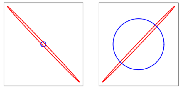
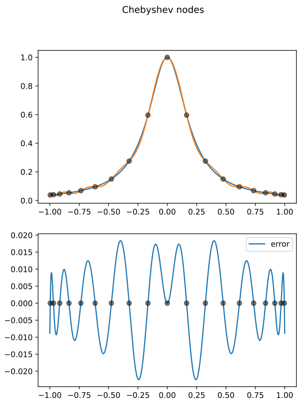
How good is cubic spline interpolation (with "natural" end conditions) for Runge's function using 19 uniformly spaced points on [-1,1] (including the endpoints)? For comparison, the degree-19 polynomial interpolant using 19 uniformly spaced nodes is REALLY bad, as measured by the L^∞-norm of the discrepancy, but using Chebyshev nodes is much better: see pictures below. Support your answer with numbers and/or plots generated using the code I demonstrated in class on Day 15.

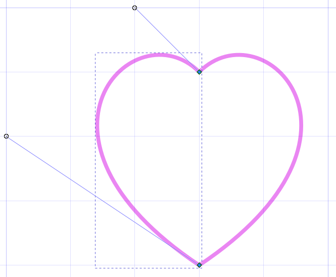
7. Bézier cubic curves

If we wanted to draw an approximate circle with Bézier cubics, we might try doing it in 4 pieces, approximating the quarter-circle {(cosθ, sinθ) | θ ∈ [0, π ⁄ 2} with a Bézier segment. In that case it seems that we'd have to have P₀ = (1, 0) and P₃ = (0, 1), and for the approximate circle not to have a corner at the segment ends, we'd need a vertical tangent at P₀, and a horizontal tangent at P₃. Thus P₁ should be directly above P₀: P₁ = (1, something) and P₂ directly to the right of P₃: P₂ = (something, 1). And for symmetry we'd also need those two somethings to be the same. Thus it seems like we have only one degree of freedom: the value of "something". By trial-and-error, or other means, find a good value. Explain how you came up with your answer, make a plot of your approximate circle, and give some measure of its deviation from a perfect circle.

1. Bounded total variation?

Theorem 4.16 on p 251 has a hypothesis that the function has "bounded total variation" - see Def 4.19 on the previous page. Consider the functions f₅(x) = x − x², f₆(x) = ⎧⎨⎩ x sin(1 ⁄ x),  x ≠ 0     0,  x = 0  .

For each function,

1. Is f_i ∈ C¹[0, 1]?

b. Does f_i have bounded total variation on the interval [0,1]? If not, give a specific sequence of partitions for which the variation is unbounded. If so, prove that the sup of the variation wrt all partitions is whatever it is.

2.

1. Invent a function f : [0, 2π) → ℝ whose periodic extension to ℝ is in C³ but not in C⁴.

b. Use the code from Day 16 to draw ||g_k − f||_∞ for k = 1, 2, ..., 10, on a log-log plot and comment on the agreement or otherwise with Thm 4.17. NOTE You will need to change "quadrature" to "quad" and add the argument complex_func=True. See this for more details - thanks, Joel!.

3.

Do the following by hand.

1. What is the matrix of the discrete Fourier transform F₄ (Ackleh version - see Day 17) for n = 4, expressed explicitly and as simply as possible?
2. What is the matrix of the inverse F^− 1₄ (explicitly and as simply as possible)?
3. What is the DFT of the vector y = [3, 1, 1, 3]^T (explicitly and as simply as possible)?

d. What is the band-limited trigonometric interpolant of the data in part c, if the y_i are the values at x = 0L ⁄ 4, 1L ⁄ 4, 2L ⁄ 4, 3L ⁄ 4? I recommend you plot your answer to see if it's correct.

4. Operation count for fast fourier transform

The way I've coded it in the class notes from Day 18 = Day -12, the number of operations C_n to do the DFT of size n is:

• 1 division and an exponentiation to form w - call that 2 ops
• n-1 multiplications to form the vector W (I could do it with that few, if I tried.)
• 2 C_{n/2} to do the two smaller DFTs
• n multiplies and n adds to get the answer

That's a total of 2C_n ⁄ 2 + 3n + 1 operations, and we have the recurrence relation C_n = 2C_n ⁄ 2 + 3n + 1 with starting condition C₁ = 0. This relation tells us C₂ = 2(0) + 3*2 + 1 = 7, C₄ = 2(7) + 3*4 + 1 = 27, and [C₁, C₂, C₄, C₈, ...] = [0, 7, 27, 79, 207, 511, ...].

1. Forward and reverse mode automatic differentiation

By hand, exhibit the computation of the value and derivative of the expression (x³)/(8 − x) at x = 3, (a) using forward-mode AD, and (b) using reverse-mode AD. [Note to self: better if use different value of x so that x^3 != 3x^2.]

NOTE: I neglected to update this as I intended before posting. Although you may do the version above, my preference is that if you haven't already done it, you do the following formula instead: (x³)/(10 − x) at x = 3.

If for reverse-mode, our diagramatic convention for subtraction is that the lower incoming branch is subtracted from the upper incoming branch, you may find it convenient to have branches crosssing in your diagram, and this is perfectly ok.

Please note that the section on reverse-mode AD in the textbook is completely wrong, being just forward mode in disguise.

2. Implementation of forward-mode automatic differentiation

1. Gaussian quadrature rules

By hand, derive the 3-point Gauss-Legendre quadrature rule by guessing the symmetry and requiring that it has polynomial degree 5.

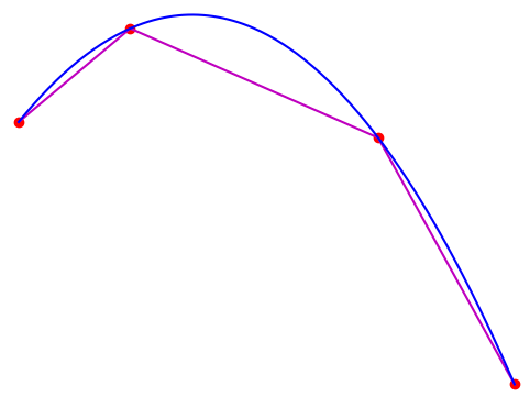
2. Using a quadrature rule

Obtain an accurate approximation to the length of this curve made of two Bezier segments, if the grid squares have side 1 meter. Be sure to specify precisely what quadrature rule(s) you are applying and any other relevant specifics of the quadrature method.

If appropriate set the error tolerances for the quadrature function, and specify the answer to a precision that is appropriate given the error estimate. Hint: If your velocity is v(t), between time a and time b you travel a distance ∫^b_a ||v(t)|| dt. Note: It is a rare curve for which this integral for its length can be evaluated by antidifferentiation.

3. Newton's methods for systems of (nonlinear) equations

(a) By hand, and showing all steps, perform a single iteration of Newton's method on the system "Ex 1" considered in class on Nov 21, and starting at [u,v] = [1,2].

2. Compute the Broyden update of the jacobian using the value of F at the new point, and compare with the actual jacobian at the new point and comment.

4. Efficiency in Newton's method

1. Verify the Sherman-Morrison formula for updating the inverse of a matrix subject to a rank-1 change.
2. Explain why the Sherman-Morrison update does not entail any O(n³) matrix-matrix multiplications.

Optimization in multiple dimensions

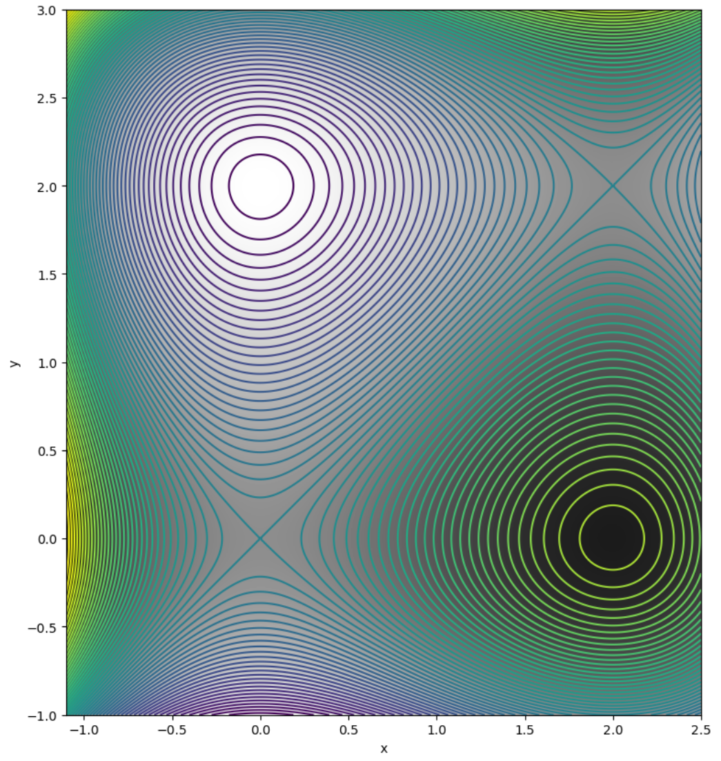
1. Consider the problem of finding a local minimizer of the function f(x, y) =  − x³ + y³ + 3x² − 3y² + 12.

(a) By hand, and showing all your steps, calculate the formula for f along the initial 1D line search - in either steepest descent or conjugate gradient methods - starting at (x,y) = (-1,1), and find the local minimizer closest to your starting point.

(b) For the starting point (-1,1), doing no computation and using only the information provided by the level curves in the plot, by hand sketch on the following contour plot of f (i) the first 3 steepest-descent line minimizations, (ii) the curve resulting from following the local gradient at every point. Recall that the gradient is orthogonal to the level curves.

3. Starting at (-1,1), compute the first step of Newton's method applied to ∇f. Show all your work.

2. We saw in class on Day 26 that McKinnon has provided an example of a function and an initial simplex for which the Nelder-Mead downhill simplex method fails - converging to a point where the gradient of the objective function is not zero. We'd want to know if this is a really special case, or if the method fails on a set of positive measure in the space of reasonable problems we might want to apply it to. Using the code I provided in class, apply the method to the McKinnon example again but with slightly perturbed initial simplexes, and determine empirically whether or not the initial simplex has to be very specially contrived for the method to fail. Describe and display what you observe, and draw your own conclusions.