438/538 Lecture Notes
Contents
- Ordinary Differential equation initial value problems
- Error in approximate solutions
- Q&A (Quiz 1)
- A more accurate method: Improved Euler
- Systems of Differential Equations
- Q&A (Quiz 2)
- Systems of ODEs, cont'd
- Taylor series method
- ODE IVP error estimation and control
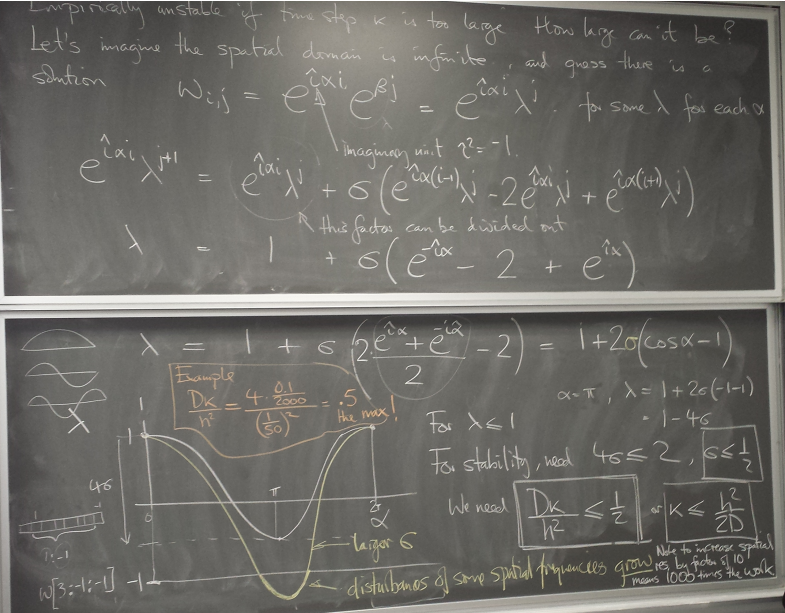
- Stiff systems and stability of methods
- Q&A (Quiz 3, Feb 4)
- Instability
- Implicit methods
- High-quality ODE integrator codes in scipy
- Multistep methods
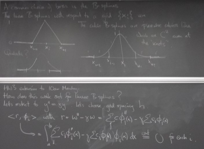
- ODE boundary value problems
- Partial Differential Equations
- Methods for parabolic PDE, cont'd
- Finite difference method for hyperbolic PDE
- Finite difference method for elliptic PDE
- Iterative methods for sparse linear systems
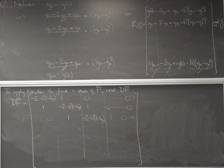
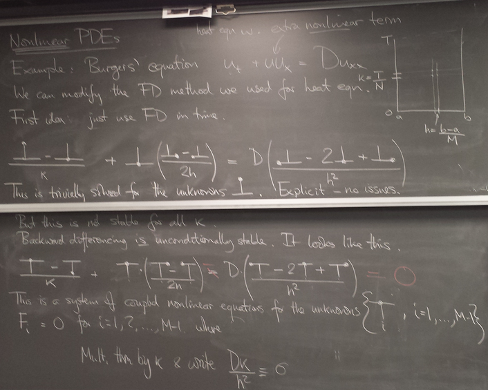
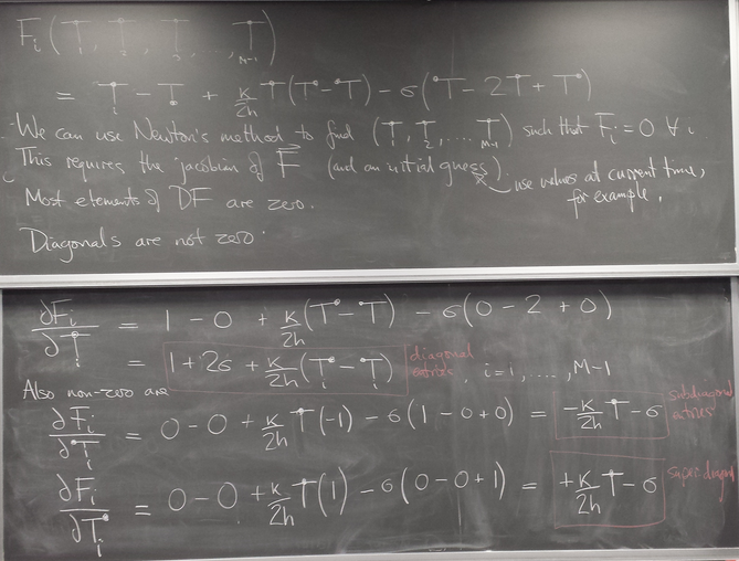
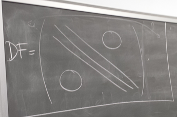
- Nonlinear PDE
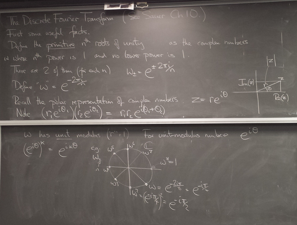
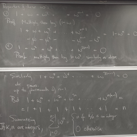
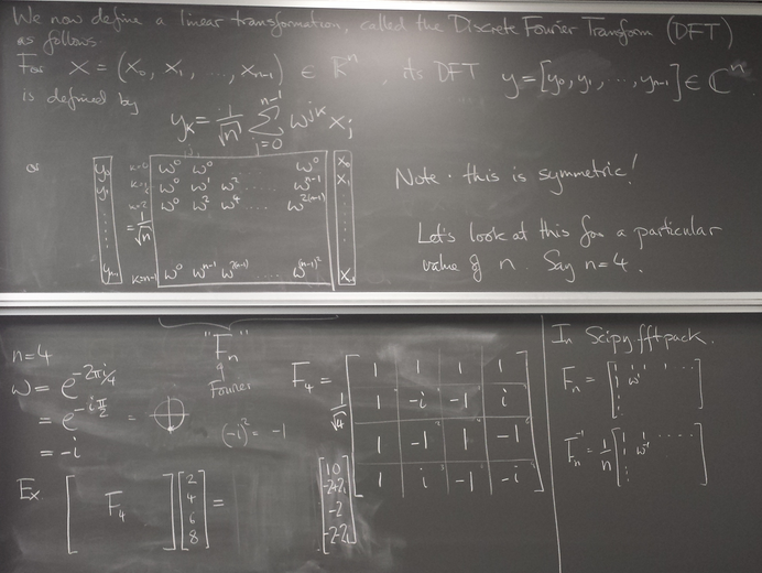
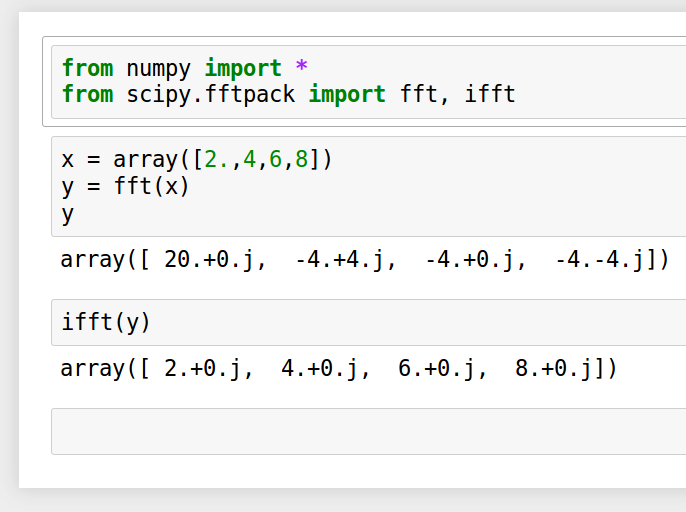
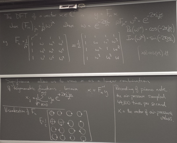
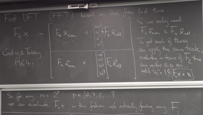
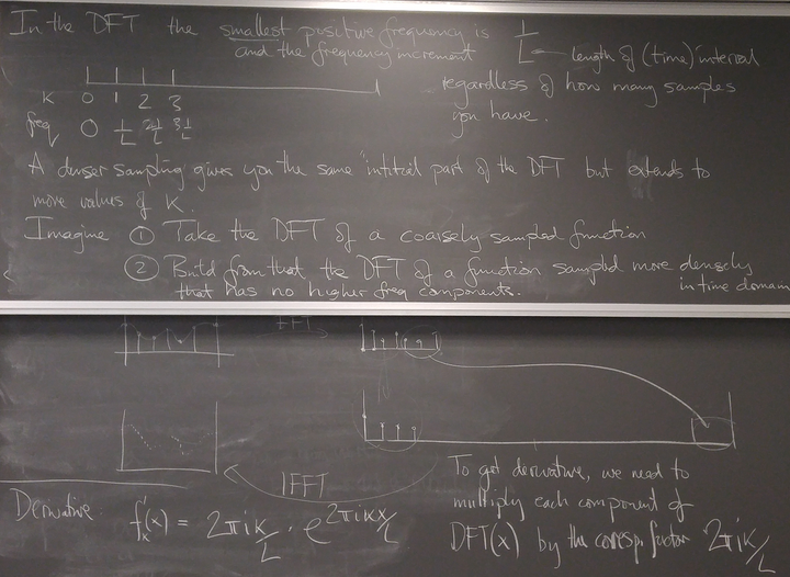
- Discrete Fourier Transform
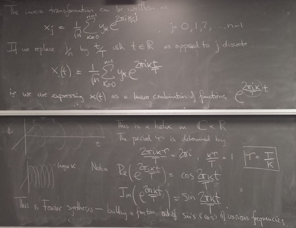
- Discrete Fourier Transform, cont'd
- Project selections
- Fast Fourier Transform, cont'd
- Trigonometric Interpolation
- Exam 2
- Trigonometric interpolation, cont'd
- Spectral differentiation
- Exam 2
- Homework Assignment 7 review
- Spectral derivatives, cont'd
- Computing eigenvalues and eigenvectors of matrices
- Visualizations for project presentations
- Project presentations
- Eigenvalues and eigenvectors, conclusion
- Singular Value Decomposition (SVD)
- Online course evaluations
Tuesday, Jan 26, 2016
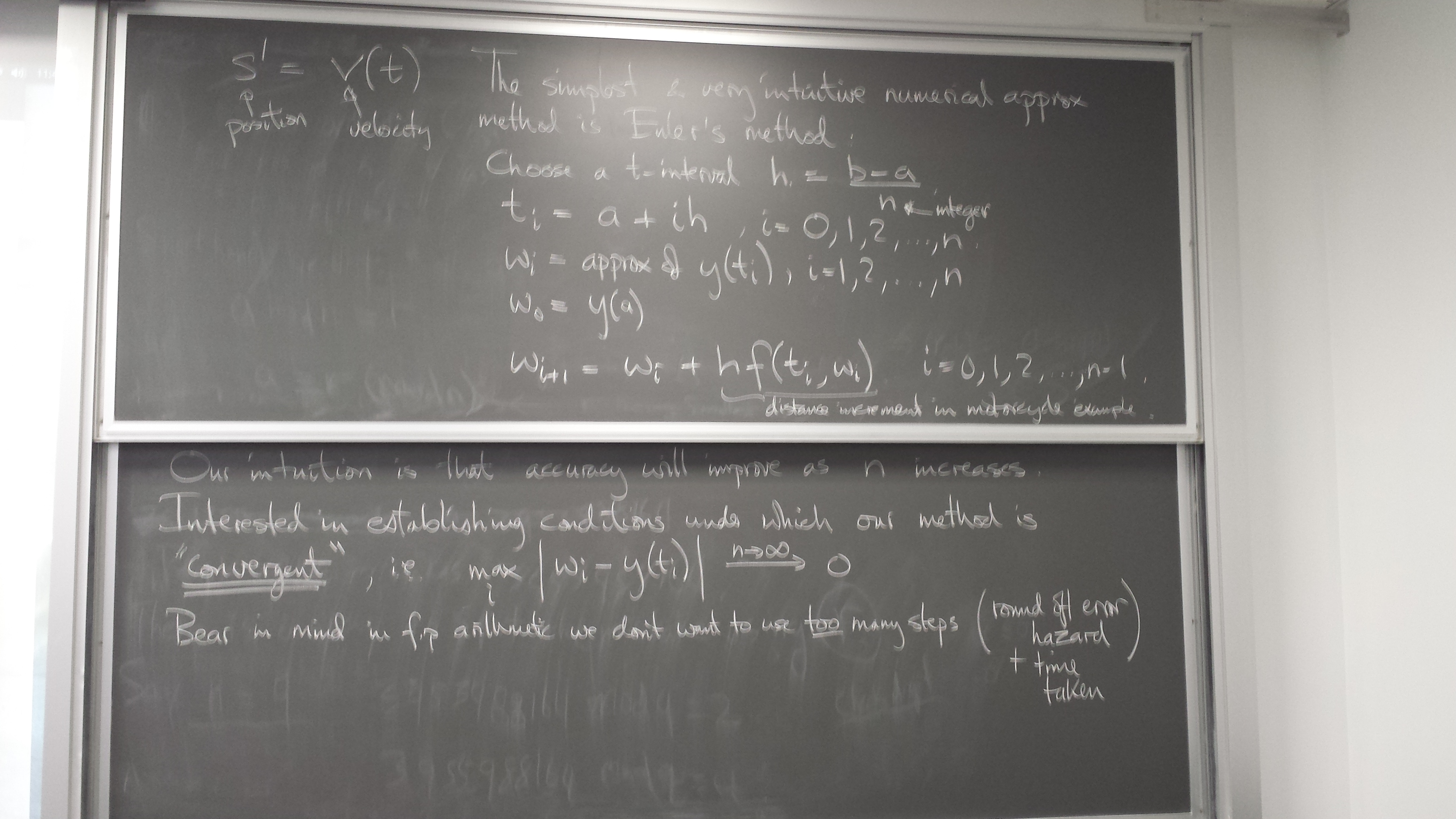
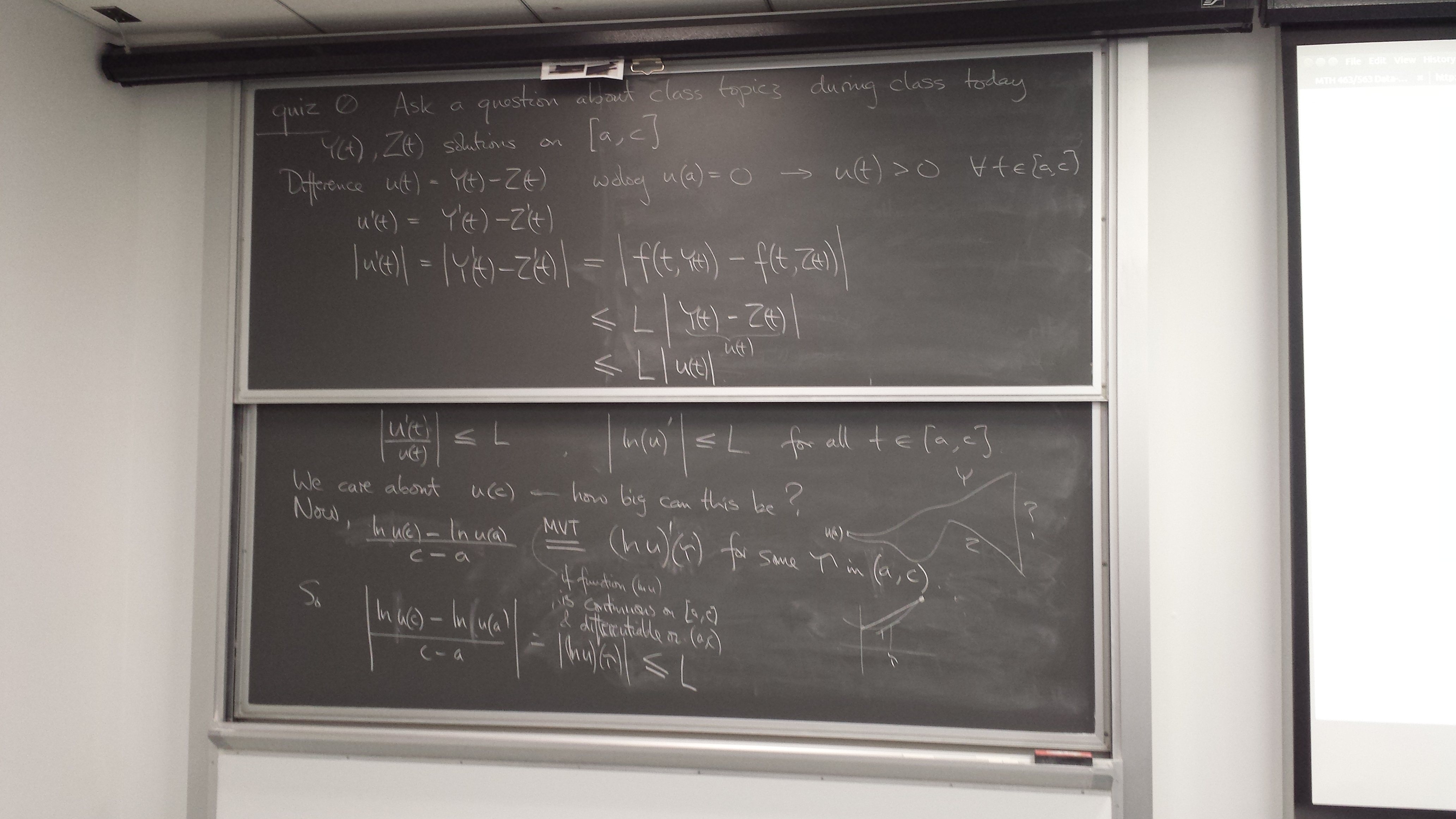
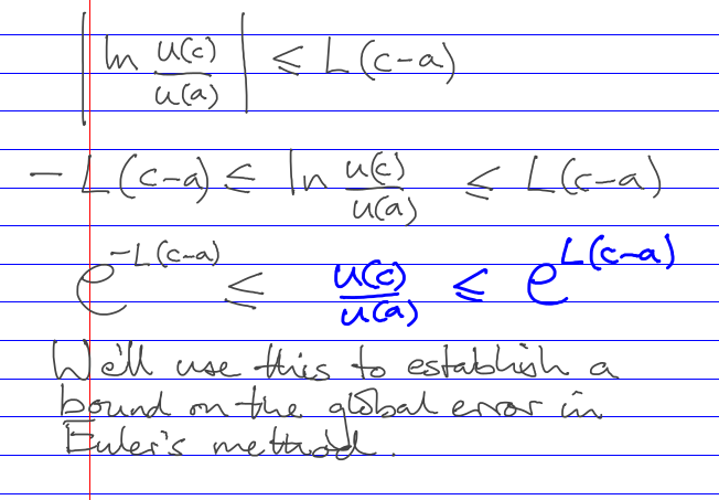
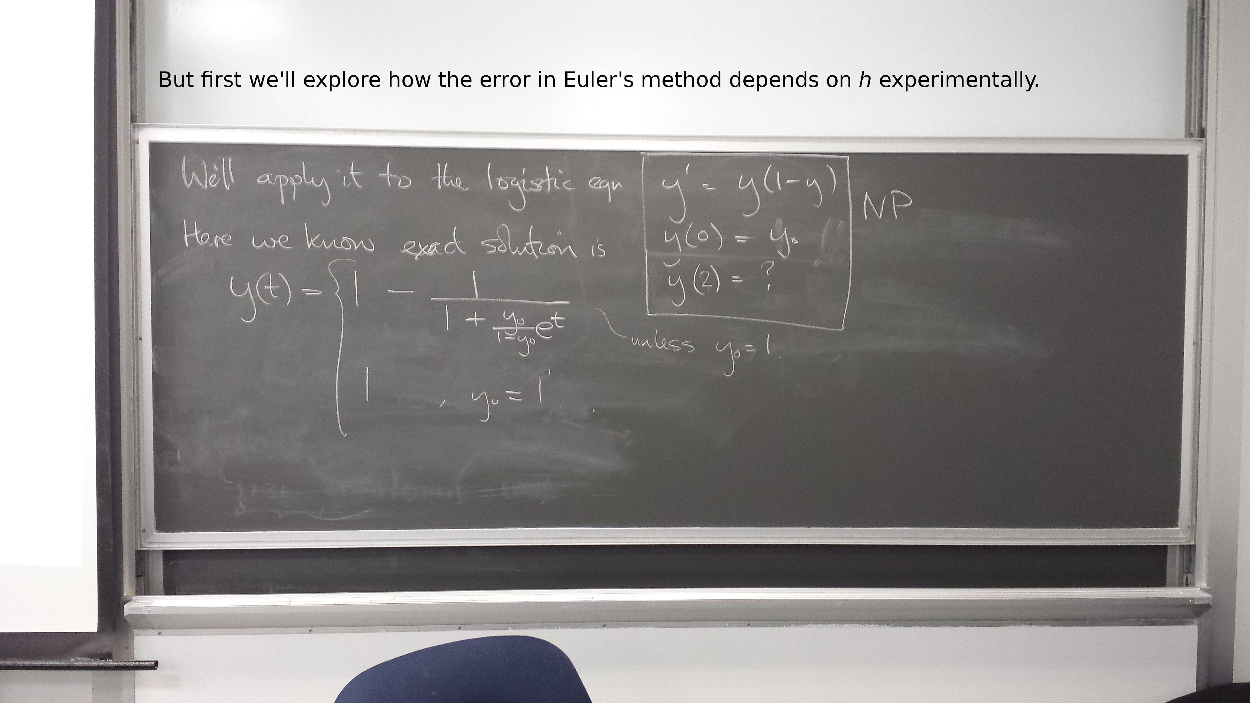
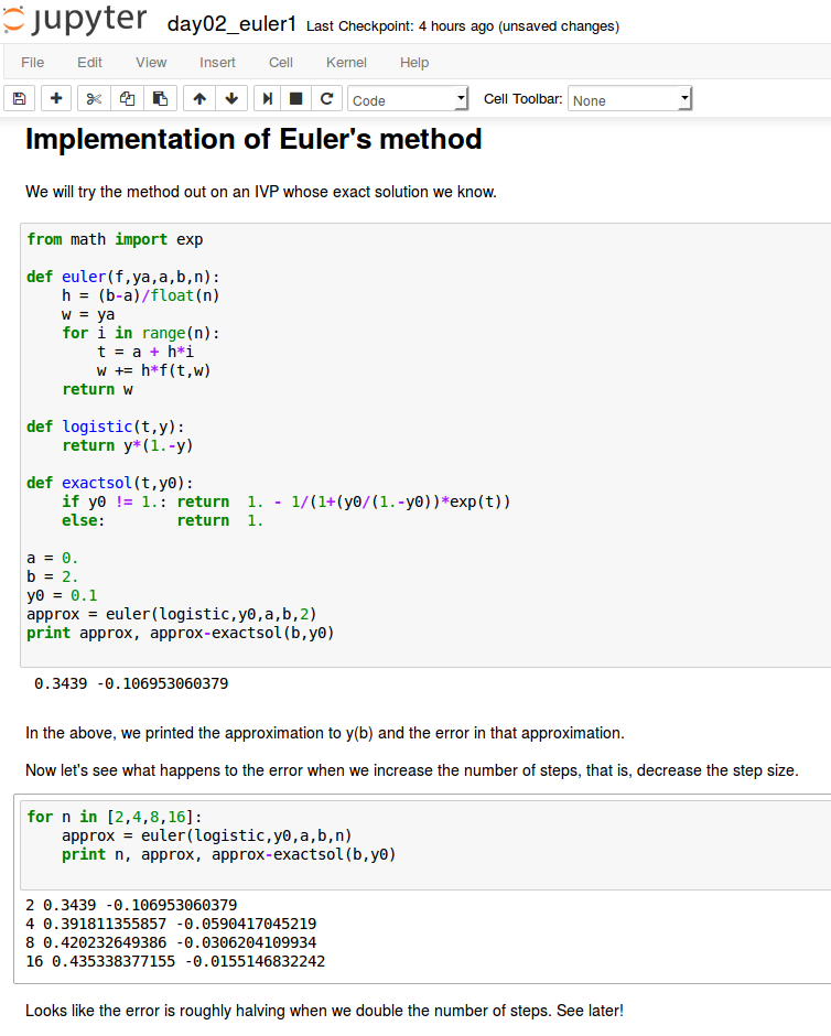
Ordinary Differential equation initial value problems
What an ODE IVP and its solution are

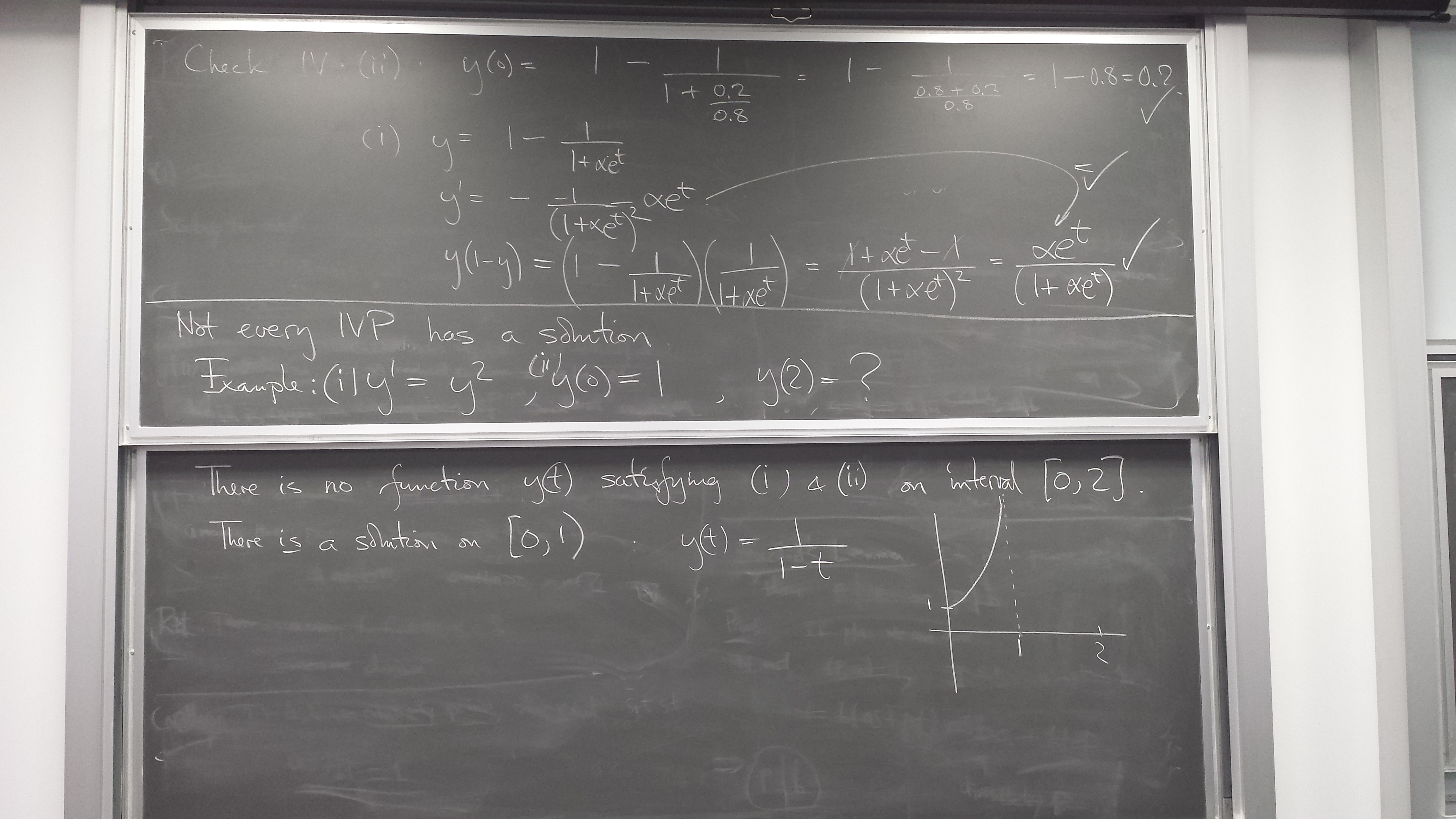
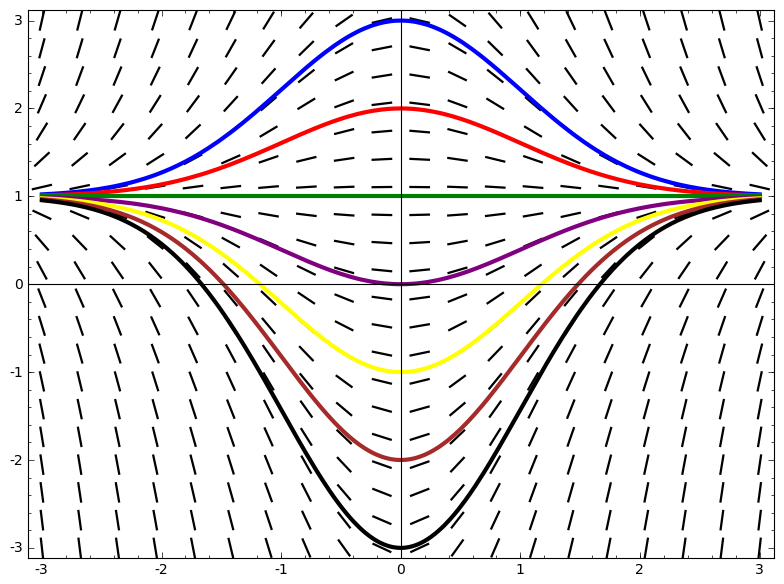
Slope field - the information content of a differential equation y' = f(t,y)
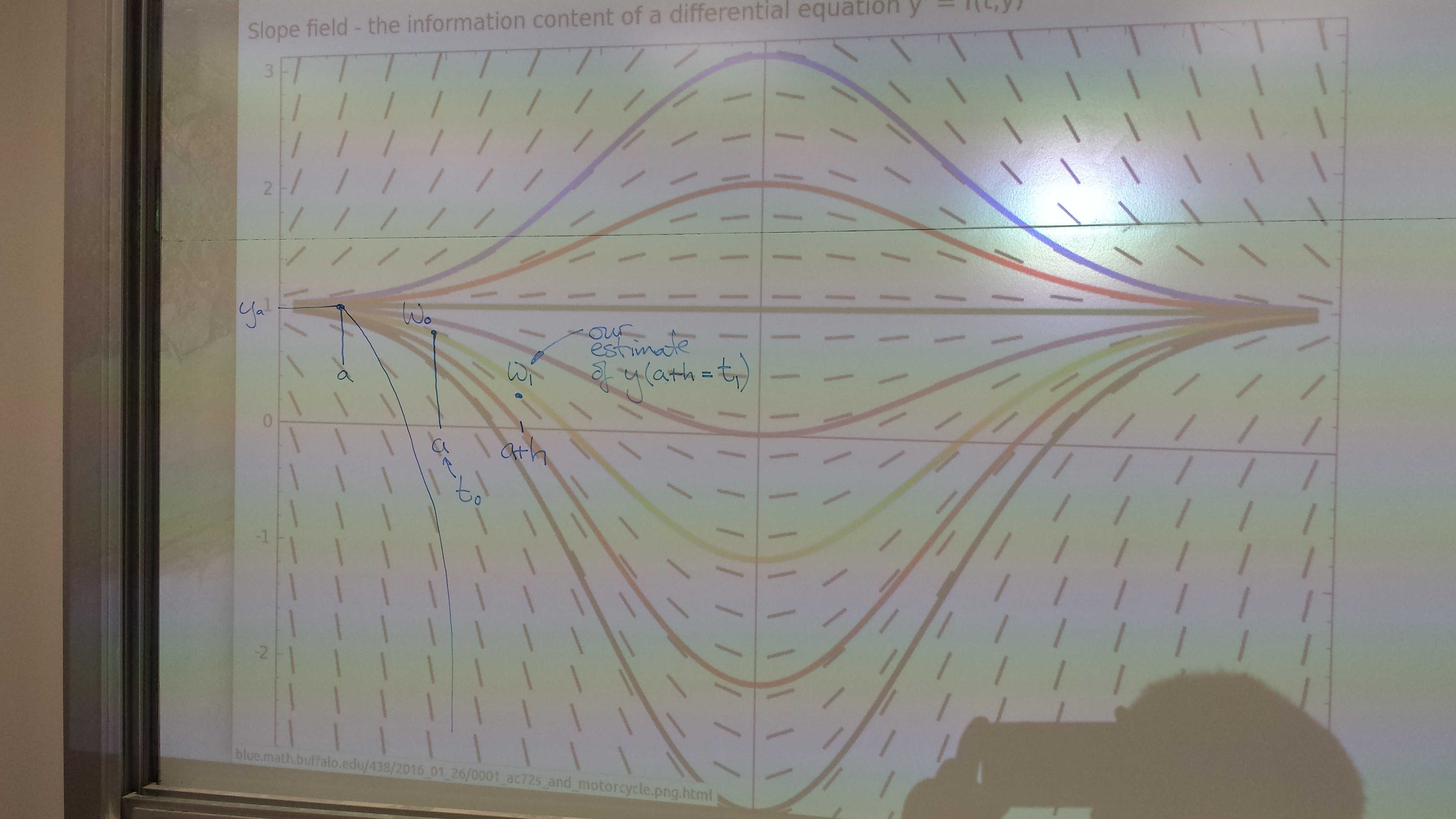
Euler's method
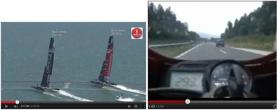
How far will these boats and this motorcycle travel: (i) in the next minute? (ii) in the next second?

Q&A (Quiz 1)
Nigel asks:
Sean asks:
Sun asks:
Deanna asks:
Gary asks:
Neil asks:
Jackson asks:
Thomas asks:
Dante asks:
Jonathan asks:
Nathan asks:
Tiehang asks:
Tuesday, Feb 2, 2016
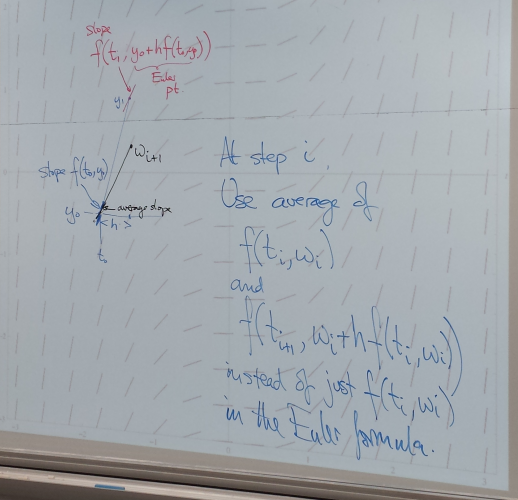
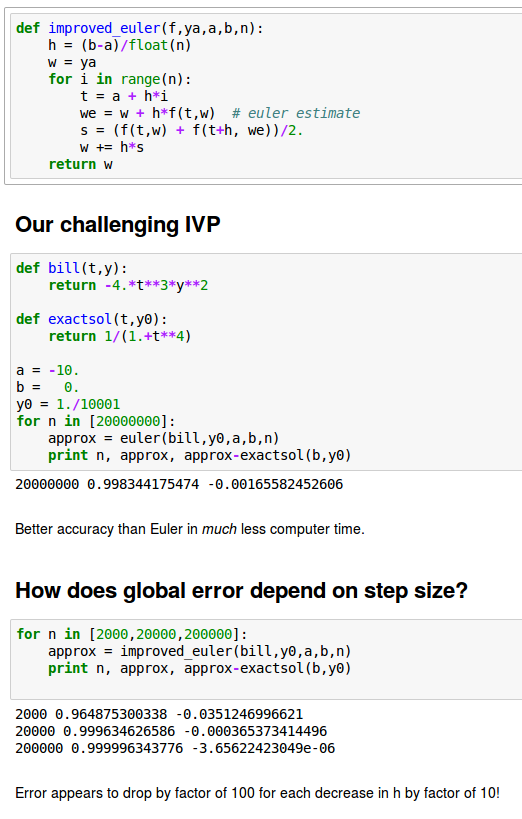
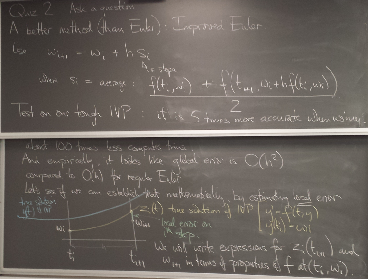
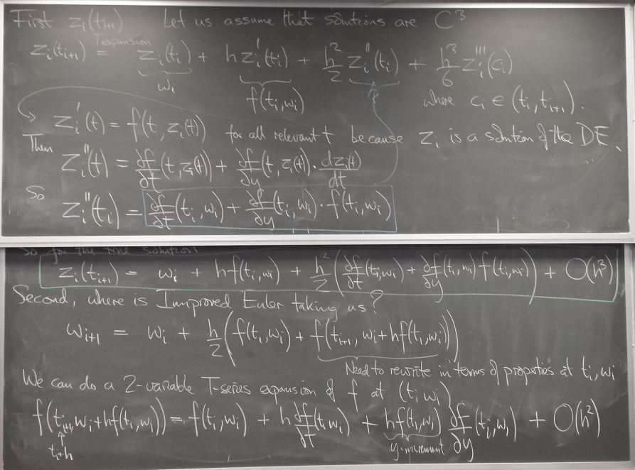
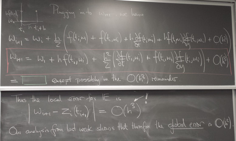
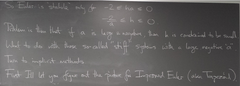
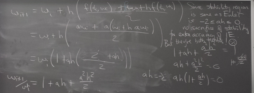
A more accurate method: Improved Euler
a.k.a. Trapezoid method
A method with local error of higher order in h, O(h^3), is obtained by "looking ahead".
We take a modified Euler step using the average of the slopes at the current point and at the point where the regular Euler step takes us.
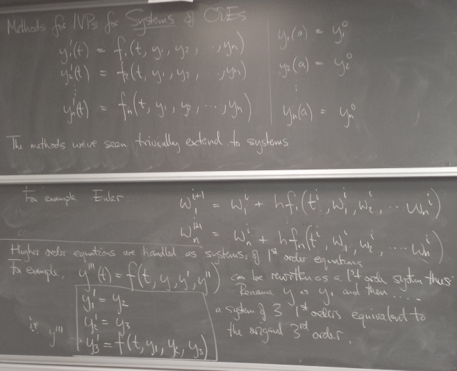
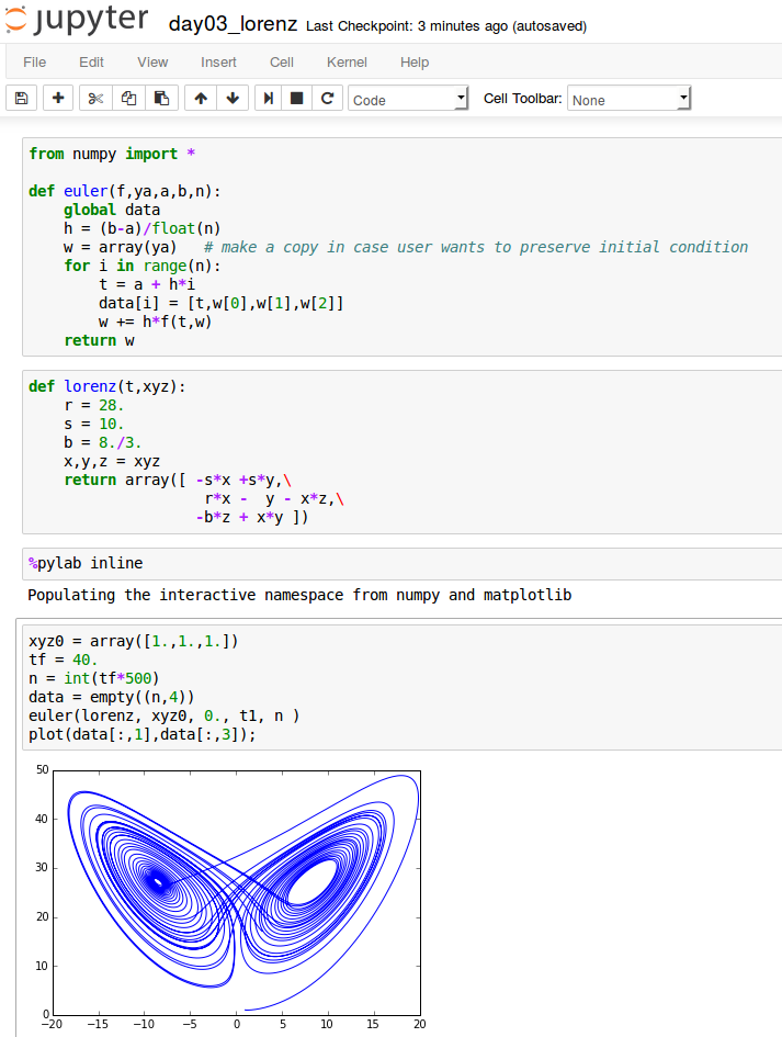
Systems of Differential Equations
Systems of coupled first-order DEs can be handled by simply vectorizing the previous methods.
Higher-order DEs can also be handled in this way - by converting them to systems of first-order DEs.
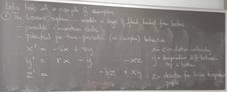
Example: Lorenz system
A system of 3 coupled ODEs that coarsely models a tank of fluid heated from below.
Q&A (Quiz 2)
Jonathan Lottes asks:
Nigel Michki asks:
David Bryant asks:
Sun Kim asks:
Deanna Rudik asks:
Neil Heinzer asks:
Sean Moran asks:
Dante Iozzo asks:
Gary Bolduc asks:
Nathan Margaglio asks:
Jackson Donnelly asks:
Thomas Schouten asks:
Anpeng Zhang asks:
Runpu asks:
Thursday, Feb 4, 2016
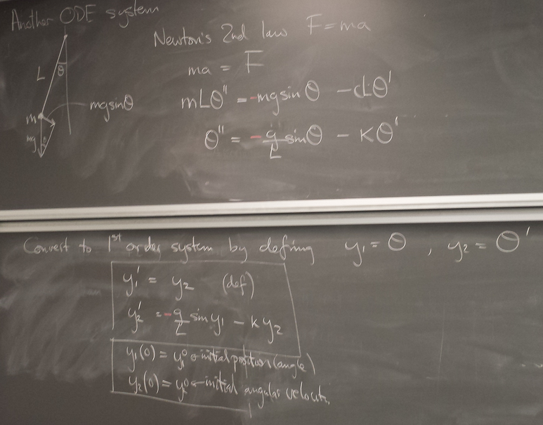
Systems of ODEs, cont'd
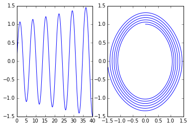
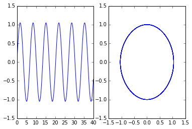
Example: pendulum
A nice test of accuracy, because we know analytically that bounded orbits are ellipses.
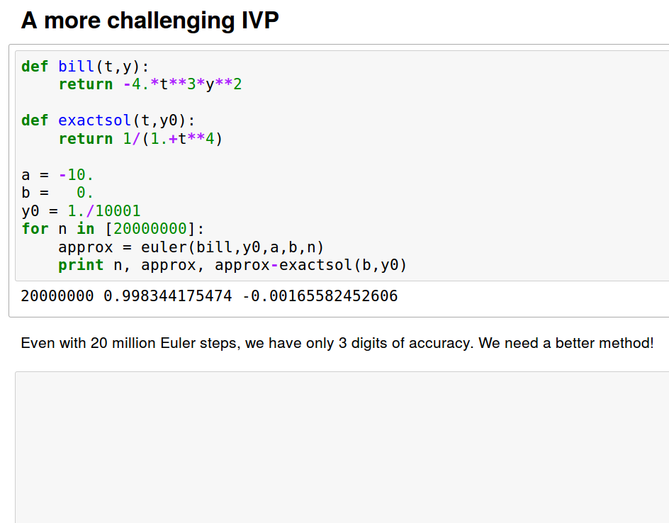
from numpy import *

def euler(f,ya,a,b,n):
    global data
    h = (b-a)/float(n)
    w = array(ya)   # make a copy in case user wants to preserve initial condition
    for i in range(n):
        t = a + h*i
        data[i] = [t,w[0],w[1]]
        w += h*f(t,w)
    return w

def improved_euler(f,ya,a,b,n):
    h = (b-a)/float(n)
    w = array(ya)
    for i in range(n):
        t = a + h*i
        data[i] = [t,w[0],w[1]]
        we = w + h*f(t,w)  # euler estimate
        s = (f(t,w) + f(t+h, we))/2.
        w += h*s
    return w
def pendulum(t,y1y2):
    g = 1.
    L = 1.
    k = 0.  # no friction to start with
    y1,y2 = y1y2
    return array([ y2, -g/L*sin(y1) - k*y2 ])
%pylab inline
Populating the interactive namespace from numpy and matplotlib
y1y20 = array([0,1.])
tf = 40.
n = int(tf*50)
data = empty((n,3))
euler(pendulum, y1y20, 0., tf, n )
subplot(1,2,1)
plot(data[:,0],data[:,1]);  # y1 vs t
subplot(1,2,2)
plot(data[:,1],data[:,2]);  # y2 vs y1
y1y20 = array([0,1.])
tf = 40.
n = int(tf*50)
data = empty((n,3))
improved_euler(pendulum, y1y20, 0., tf, n )
subplot(1,2,1)
plot(data[:,0],data[:,1]);  # y1 vs t
subplot(1,2,2)
plot(data[:,1],data[:,2]);  # y2 vs y1
Animation
This translation of a Sauer code animates the solution of the pendulum equation with some friction added.

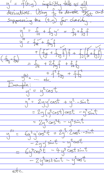
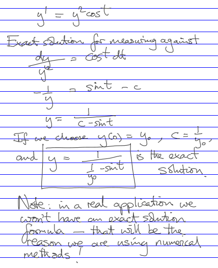
Taylor series method
So far, we've used only the slope (first derivative) given to us explicitly by the differential equation
But the DE implicitly also tells us all the higher order derivatives of a solution, and we can use that information to construct a more accurate high-order approximation without the look-ahead of the Improved Euler method.
Practice
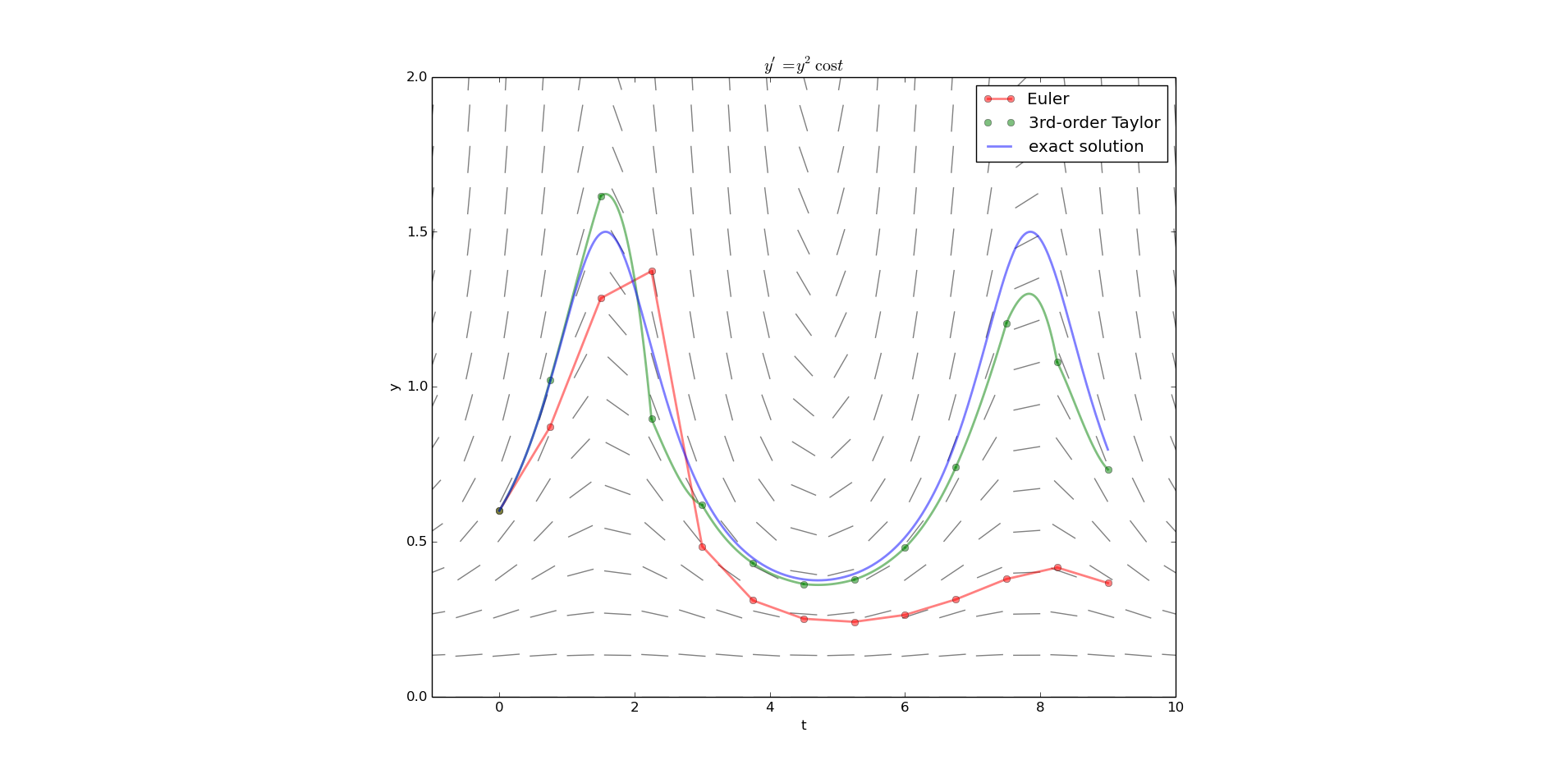
from pylab import plot,show,xlabel,ylabel,savefig,legend,title
from numpy import array,cos,sin,linspace,empty
from dfield import dfield
import sys

def yprime(t,y): return y**2 * cos(t)  # the RHS of the differential equation

def taylorcoeffs(t,y):
        c = cos(t)
        s = sin(t)
        yp   = y**2 * c
        ypp  = 2*y**3*c**2 - y**2*s
        yppp = 6*y**4*c**3 - 4*y**3*c*s - 2*y**3*c*s - y**2*c
        return y, yp, ypp/2., yppp/6.

def evaltaylor(coeffs,h):
        return sum( [coeffs[i]*h**i for i in range(len(coeffs)) ] )

def exactsolution(t,a,ya):
        c = 1./ya + sin(a)
        return  1/(c-sin(t))

a,b =  0.,9.
ya =  0.6

n = 12

dfield( yprime, a-1,b+1, 0,2 )

h = (b-a)/float(n)
t = linspace(a,b,n+1)

# Euler
y = empty(n+1)
y[0] = ya
for i in range(n):
        y[i+1] = y[i] + h*yprime(t[i],y[i])
plot( t, y, 'ro-' , label='Euler',linewidth=2,alpha=0.5)

# Taylor
y = empty(n+1)
y[0] = ya
for i in range(n):
        coeffs = taylorcoeffs(t[i],y[i])
        y[i+1] = evaltaylor(coeffs,h)
        #tt = linspace(t[i],t[i]+1.5*h,50)
        #plot(tt,evaltaylor(coeffs,tt-t[i]),'g')
        tt = linspace(t[i],t[i]+    h,50)
        plot(tt,evaltaylor(coeffs,tt-t[i]),'g', linewidth=2,alpha=0.5)
plot( t, y, 'go' , label='3rd-order Taylor',alpha=0.5)


tt = linspace(a,b,401)
plot( tt, exactsolution(tt,a,ya), 'b',linewidth=2,alpha=0.5, label='exact solution' )
xlabel('t')
ylabel('y')
title('$y^\prime = y^2 \cos t$')
legend()
savefig(sys.argv[0]+'.png')
show()
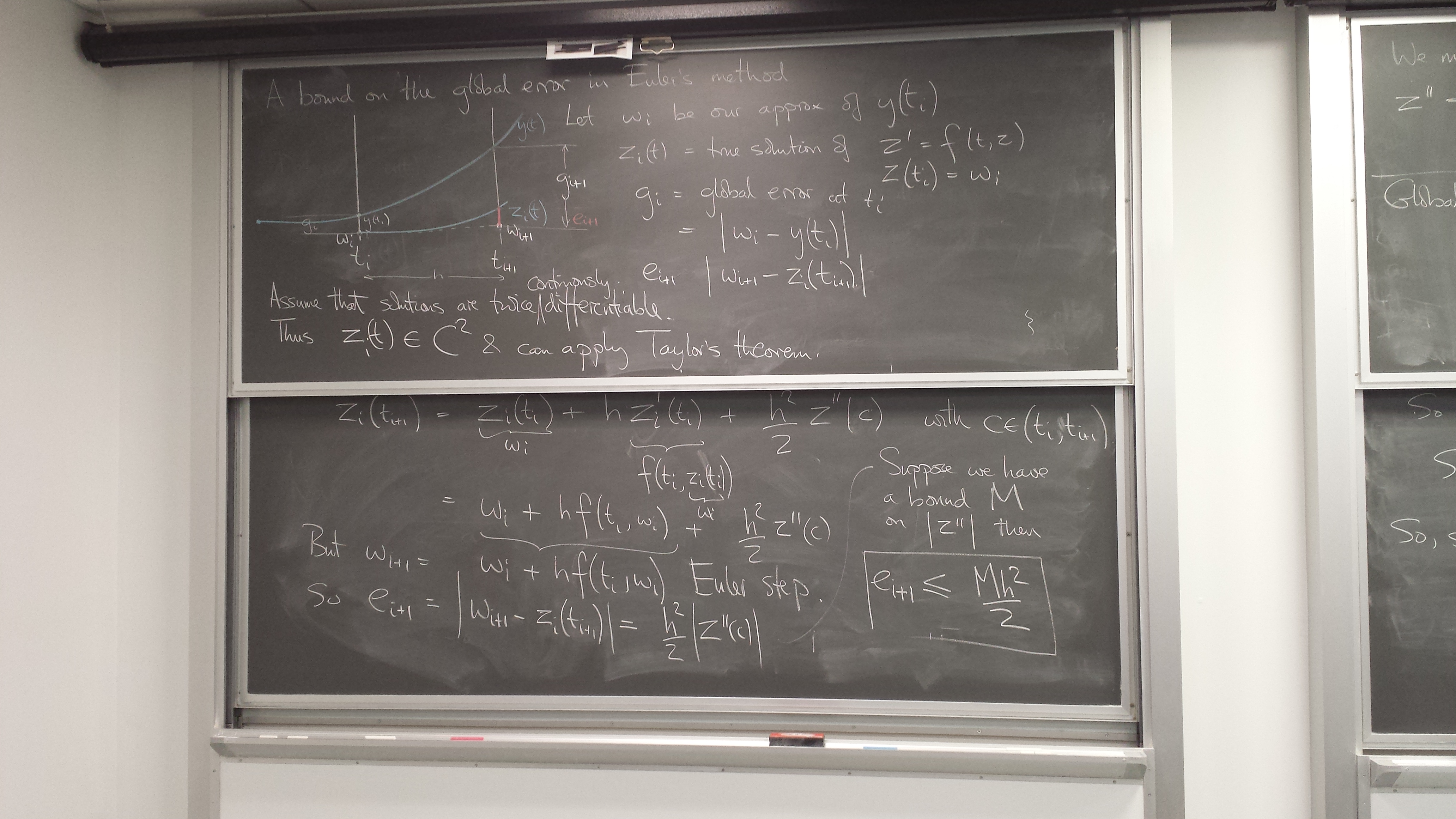
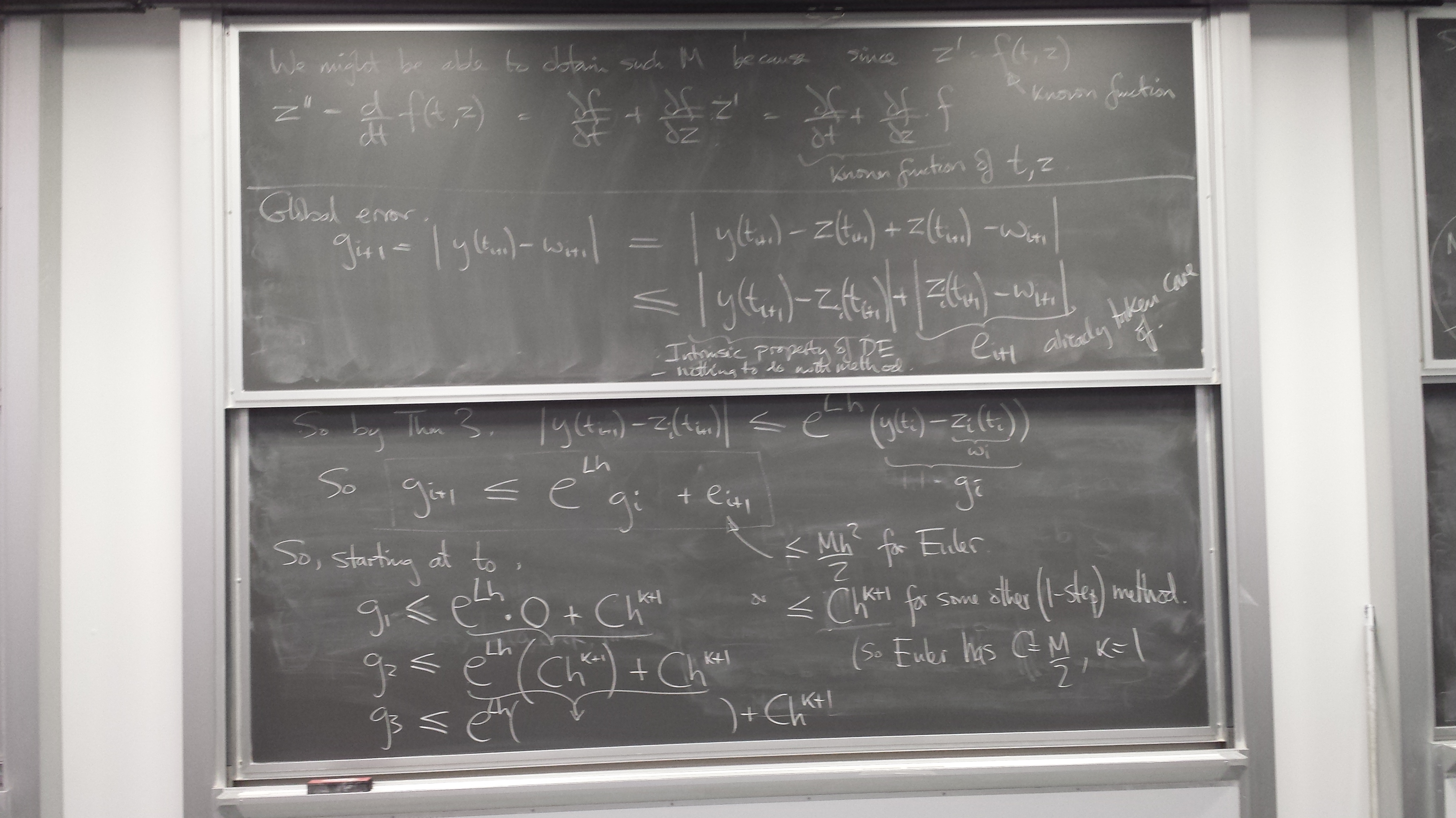
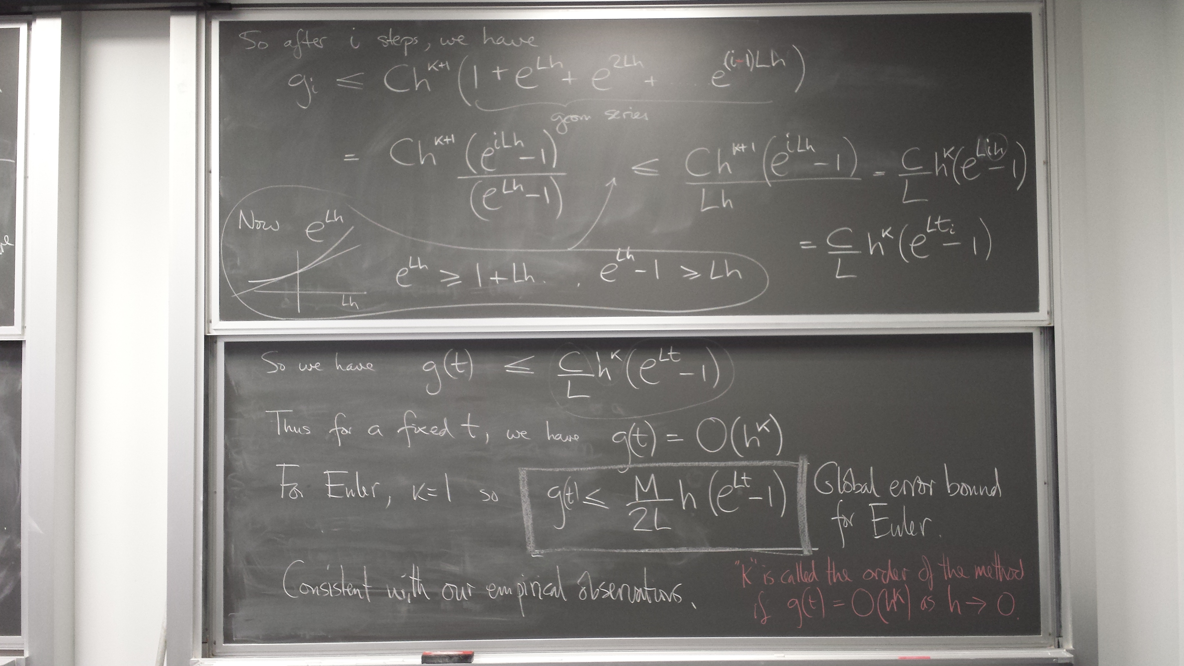
ODE IVP error estimation and control
Global error control by doing the whole thing with several fixed steps
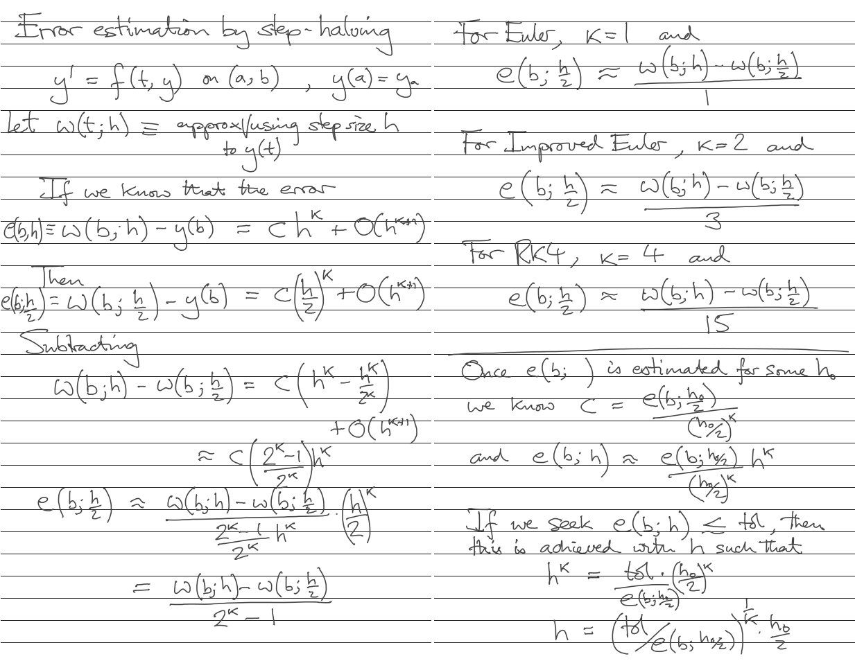
Practice
from math import ceil
def get_minimal_n(f,a,b,ya,n,method,k,tol,fsol):
    # Note the true solution fsol is not known in a real application
    wh   = method(f,a,b,ya,  n)
    who2 = method(f,a,b,ya,2*n)
    print "With",  n,"steps, solution approximation", wh,   "true value:", fsol(b,a,ya), "true error:", wh - fsol(b,a,ya)
    print "With",2*n,"steps, solution approximation", who2, "true value:", fsol(b,a,ya), "true error:", who2 - fsol(b,a,ya)
    eho2 = abs(wh-who2)/(2.**k-1.)  # estimated error in who2
    print "Estimated error with", 2*n, "steps:", eho2
    h0 = (b-a)/float(n)
    c = eho2/(h0/2.)**k
    hstar = (tol/eho2)**(1./k) * h0/2
    nmin = int(ceil((b-a)/hstar))
    return nmin
eulerk = 1
def euler(f,a,b,y0,n):
    h = (b-a)/float(n)
    w = y0
    for i in range(n):
        t = a + i*h
        w += h*f(t,w)
    return w

improvedeulerk = 2
def improvedeuler(f,a,b,y0,n):
    h = (b-a)/float(n)
    w = y0
    for i in range(n):
        t = a + i*h
        s1 = f(t,w)
        w1 = w + h*s1
        s2 = f(t+h,w1)
        w += h*(s1+s2)/2.
    return w
def f1(t,y):
    return y
from math import exp
def f1sol(t,a,ya):
    return ya*exp(t-a)
a = 0.
b = 3.
n0 = 40
ya = 4.
tol = 1.e-3

print 'Euler'
nmin = get_minimal_n(f1,a,b,ya,n0,euler,eulerk,tol,f1sol)
print 'Recommended number of steps for error of',tol,':', nmin
w = euler(f1,a,b,ya,nmin)
print "With",nmin,"steps, solution approximation", w, "true value:", f1sol(b,a,ya), "true error:", w - f1sol(b,a,ya)
print
print 'Improved Euler'
nmin = get_minimal_n(f1,a,b,ya,n0,improvedeuler,improvedeulerk,tol,f1sol)
print 'Recommended number of steps for error of',tol,':', nmin
w = improvedeuler(f1,a,b,ya,nmin)
print "With",nmin,"steps, solution approximation", w, "true value:", f1sol(b,a,ya), "true error:", w - f1sol(b,a,ya)
Euler
With 40 steps, solution approximation 72.1769558792 true value: 80.3421476928 true error: -8.16519181354
With 80 steps, solution approximation 76.0516116863 true value: 80.3421476928 true error: -4.29053600644
Estimated error with 80 steps: 3.8746558071
Recommended number of steps for error of 0.001 : 309973
With 309973 steps, solution approximation 80.3409813502 true value: 80.3421476928 true error: -0.00116634257726

Improved Euler
With 40 steps, solution approximation 80.1287989637 true value: 80.3421476928 true error: -0.213348729015
With 80 steps, solution approximation 80.2872408677 true value: 80.3421476928 true error: -0.0549068250628
Estimated error with 80 steps: 0.0528139679842
Recommended number of steps for error of 0.001 : 582
With 582 steps, solution approximation 80.34108446 true value: 80.3421476928 true error: -0.00106323277491
Adaptive step-selection to control local error
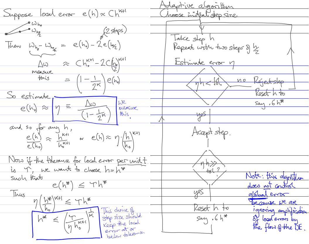
Practice
eulerk = 1
def eulerstep(f,t,y,h):
    return y + h*f(t,y)

improvedeulerk = 2
def improvedeulerstep(f,t,y,h):
    s1 = f(t,y)
    w1 = y + h*s1
    s2 = f(t+h,w1)
    return y + h*(s1+s2)/2.
from math import cos,sin
def f1(t,y):
    return y**2*cos(t)
def f1sol(t,a,ya):  # Exact solution formula: in real examples, this is not available.
    return 1./(1./ya + sin(a) - sin(t))
%pylab inline
Populating the interactive namespace from numpy and matplotlib
WARNING: pylab import has clobbered these variables: ['cos', 'sin']
%matplotlib prevents importing * from pylab and numpy
a = 0.
b = 9.
h0 = .1
ya = 0.6
globaltol = .2
tolperunittime = globaltol/(b-a)
print 'tolperunittime',tolperunittime
maxits = 1000

k = eulerk
step = eulerstep

figure(figsize=(12,10))
from dfield import dfield
dfield(f1,a-1,b+1,0.25,1.75)
tt = linspace(a,b,500)
plot(tt,f1sol(tt,a,ya),'k',alpha=0.8)
t = a
y = ya
h = h0
i = 0
safetyfactor = 0.6

while t < b:
    if i > maxits:
        print 'maxits exceeded'
        break
    i += 1
    y1  = step(f1,t     ,y  ,h   )
    y21 = step(f1,t     ,y  ,h/2.)
    y22 = step(f1,t+h/2.,y21,h/2.)
    #print y1
    #print y22
    errest = abs(y22 - y1)/(1.-1/2.**k)
    #actual_local_error = step(f1,t,y,h)-f1sol(t+h,t,y)
    #print 'errest, actual',errest,actual_local_error,actual_local_error/errest

    hstar = (h**(k+1)*tolperunittime/errest)**(1./k)
    # check validity of h*
    #actual_local_error = step(f1,t,y,hstar)-f1sol(t+hstar,t,y)
    #print 'actual_local_errorr_per_unit_t', actual_local_error/hstar


    #print 'step',h,'error estimate', errest, 'tol', tolperunittime*h
    #print 'hstar',hstar
    if errest > tolperunittime*h:
        h = safetyfactor*hstar
        #print 'reduced h to', h
    else:
        plot([t,t+h],[y,y22],'o-',alpha=0.6)
        y = y22
        t += h
        #print 'accepted step to',t,y
        if errest < 0.5*tolperunittime*h:
            h = safetyfactor*hstar
            #print 'increased h to',h
print t,y
plot(tt,f1sol(tt,t,y),'c',alpha=0.8); # backward solution from final numerical point
tolperunittime 0.0222222222222
9.05518522277 0.685998254154

The black curve is the exact solution of the IVP. The cyan curve is the backwards exact solution from the final point given by the numerical scheme. Note that the global error is not necessarily at or below the tolerance specified, due to possible amplification of the locally acceptable single-step errors by a separating flow of the DE. In this instance, the global error tolerance is satisfied, though.
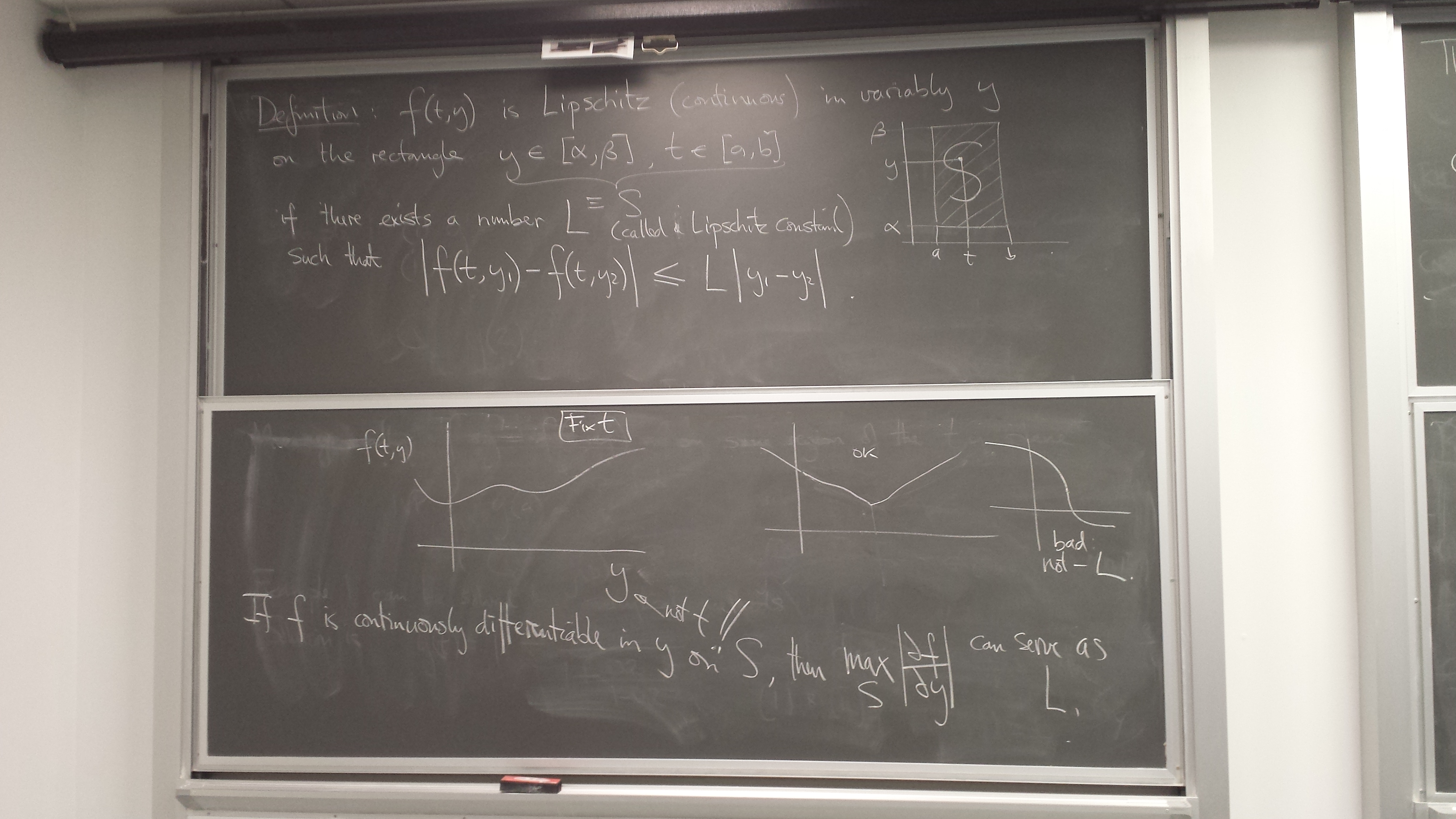
Stiff systems and stability of methods
Strong convergence of trajectories (solution curves) of a DE can cause pathological behavior - instability - of methods we've seen so far. Implicit methods can be helpful.
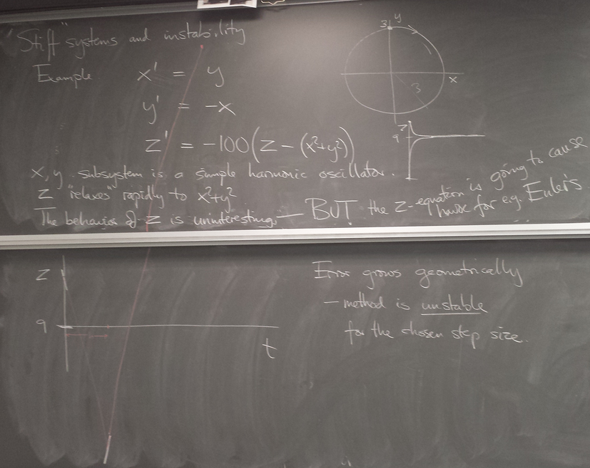
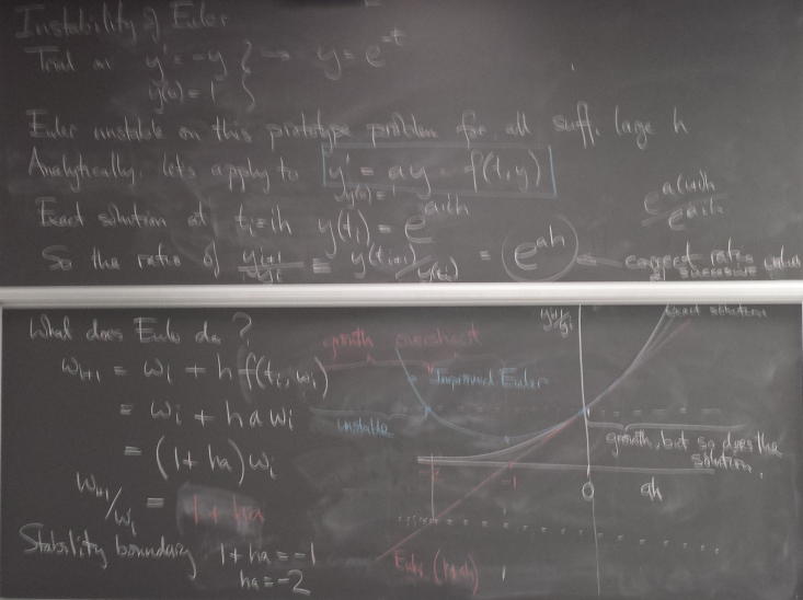
Instability of Euler's method
%pylab inline
Populating the interactive namespace from numpy and matplotlib
from numpy import *

def euler(f,ya,a,b,n):
    global data
    h = (b-a)/float(n)
    w = array(ya)   # make a copy in case user wants to preserve initial condition
    for i in range(n):
        t = a + h*i
        data[i] = [t,w[0]]
        w += h*f(t,w)
    return w
def f(t,z): return -100*(z-9)
figure(figsize=(15,8))
for n in [49,52,200]:
    z0 = array([10.])
    data = empty((n,2))
    euler(f,z0,0.,1.,n)
    plot(data[:,0],data[:,1],label='n='+str(n))
legend(loc='upper left');
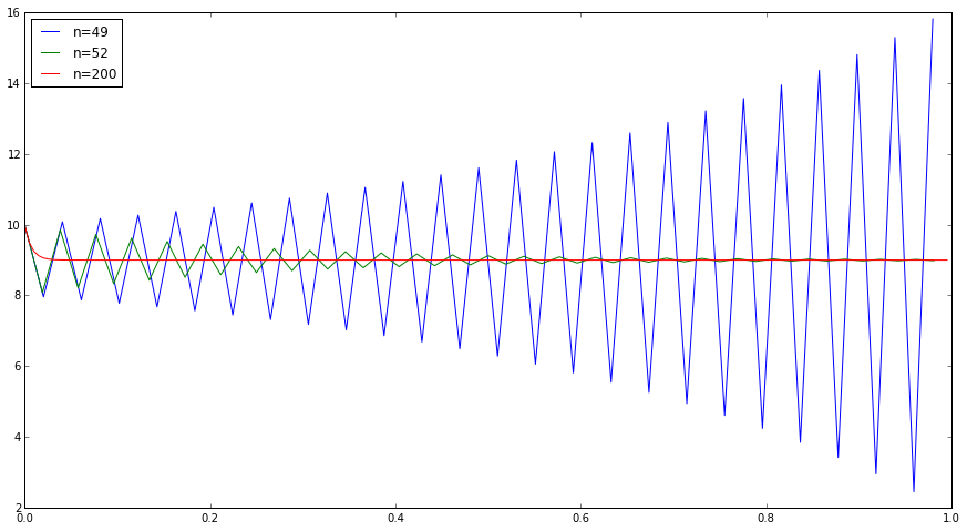
With n=200, Euler tracks the true solution quite well.
With n=52, the Euler approximation does decay asymptotically to 9, which is what the true solution does. But it does it in an oscillating fashion that is not the behavior of the true solution (which is monotonic).
With n=49, things are much worse: the Euler approximation blows up.
Q&A (Quiz 3, Feb 4)
In Quiz 3, David asks:
You mentioned that the method we used today isn't used as often as it should be. Which methods are used more often?
For a second question, why is our method (with AD or sympy) better than those methods? (time taken to find a solution lower, or just more flexibility?)
In Quiz 3, Neil asks:
In Quiz 3, Sun Hyoung asks:
In Quiz 3, Dante asks:
In Quiz 3, Thomas asks:
In Quiz 3, Nathan asks:
In Quiz 3, Eric asks:
- Why do we need to choose h = h*^k?
- Why does the "uninteresting z" create problems for Euler's method, does this also cause problems for Improved Euler as well?
In Quiz3 Question, Tiehang asks:
Anpeng asks:
Runpu asks:
Jackson asks:
Le Yang asks:
Jonathan asks:
Deanna asks:
Gary asks:
Nigel asks:
Tuesday, Jan 9, 2016 Outline
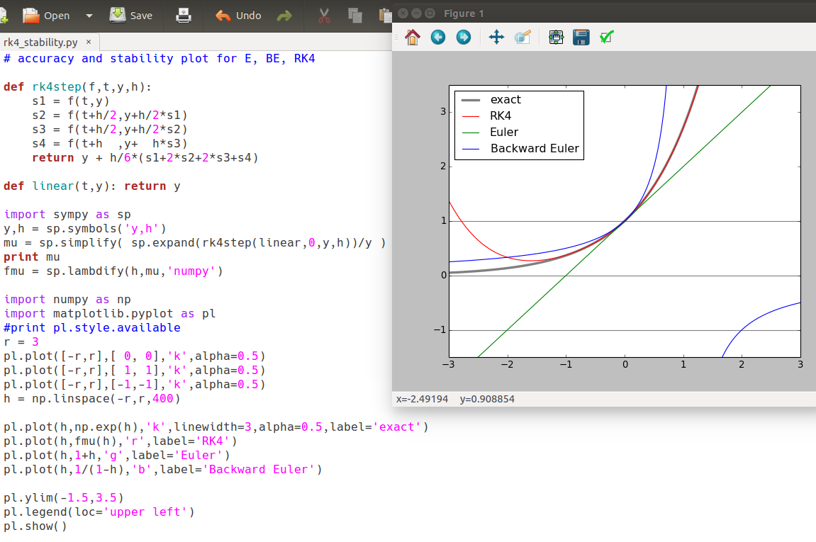
Implicit methods
Backward Euler
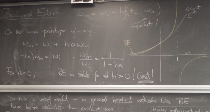
Solving the implicit relation
Nonlinear example:
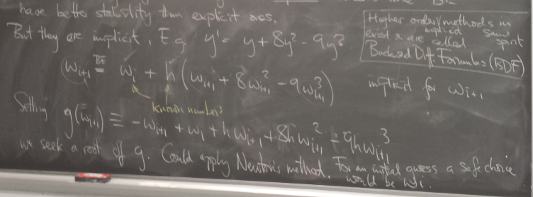
y=1 is an equilibrium. Newton can be used to solve for the BE step.
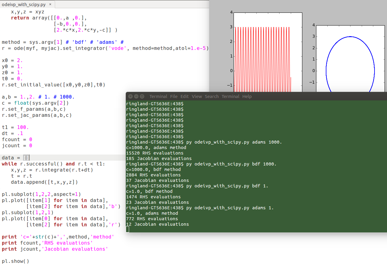
High-quality ODE integrator codes in scipy
Trying the "vode" code on the potentially stiff 3D system I introduced last time, we see that the "BDF" method is more efficient (fewer function calls) than "Adams" on a stiff problem (c=1000), while Adams is more efficient than BDF on a non-stiff problem (c=1).
Multistep methods
Derivation of formulas, and stability
The single-step (mutistage) methods we've discussed so far, like Improved Euler and Runge-Kutta methods, use multiple function evaluations at each step, "sniffing around" to gather higher order information about the DE. They completely ignore "history", except for the current value w_i.
The idea of multistep methods is to use previously gathered w's and f(t,w)'s as an alternative means for obtaining higher-order information, so that only one new function evaluation is required for each step.
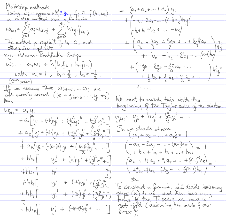
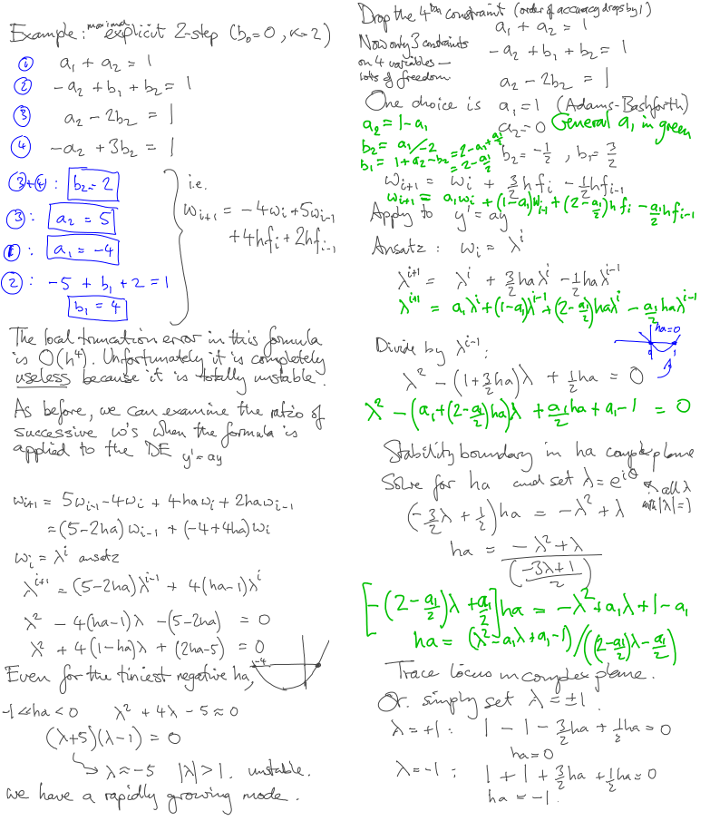
The code multistep_stability.py plots the moduli of the eigenvalues of an explicit 2-step method as a function of ha. If either of them is greater than 1, the iterates will blow up.
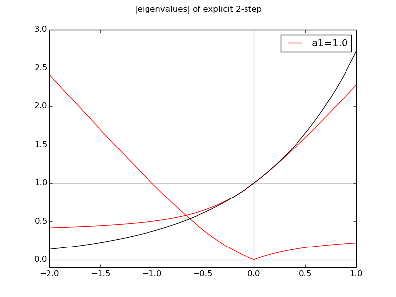
The implicit formulas (i.e. b0 not set to 0) with a1=1 are called Adams-Moulton formulas. The extra degree of freedom allows them to be of degree 1 higher than the corresponding explicit Adams-Bashforth method. An AB-AM pair of methods are often used where the explicit AB method gives a "prediction" of w[i+1], and the AM formula is applied to "correct" it.
Performance: multistep vs single-step methods
Using the same ODE as last time to test performance, we see that the "dopri5" (Runge-Kutta-like) Dormand-Prince method uses about 10 times as many function evaluations as the Adams method. This appears to justify the idea we began this section with, that making use of history is a more frugal way of obtaining higher-order information.
Non-stiff problem:
$ py odeivp_with_scipy.py dopri5 1.
c=1.0, dopri5 method
7014 RHS evaluations
0 Jacobian evaluations

$ py odeivp_with_scipy.py adams 1.
c=1.0, adams method
772 RHS evaluations
12 Jacobian evaluations
Stiff problem:
$ py odeivp_with_scipy.py adams 1000.
c=1000.0, adams method
15520 RHS evaluations
185 Jacobian evaluations

$ py odeivp_with_scipy.py dopri5 1000.
c=1000.0, dopri5 method
225588 RHS evaluations
0 Jacobian evaluations
Q&A
Jonathan asks:
Anpeng asks:
Tiehang asks:
Dante asks:
Tuesday, Feb 16, 2016
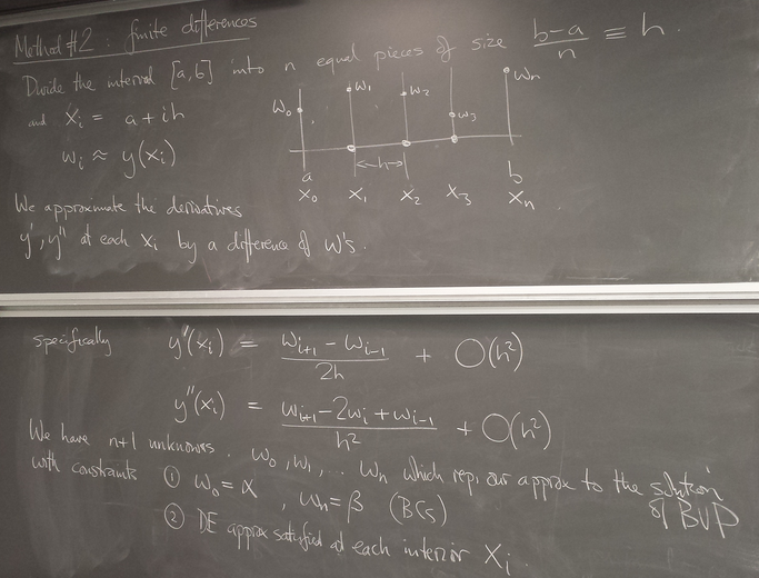
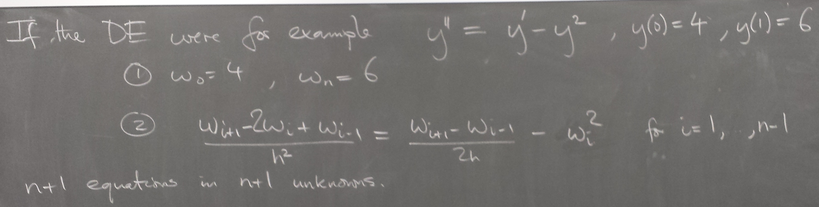
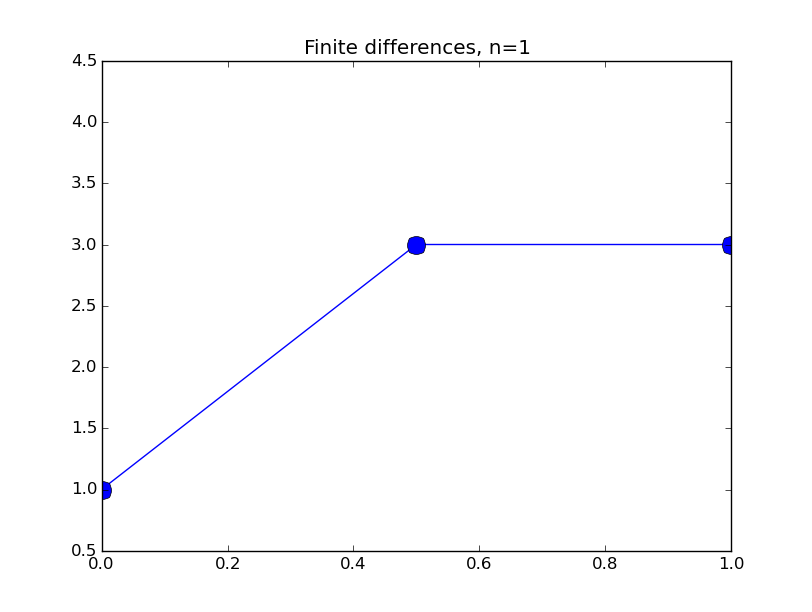
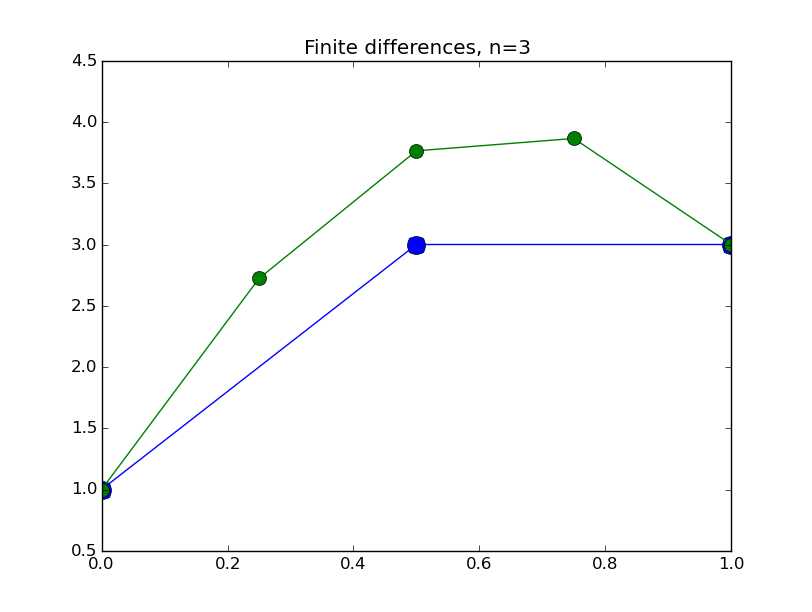
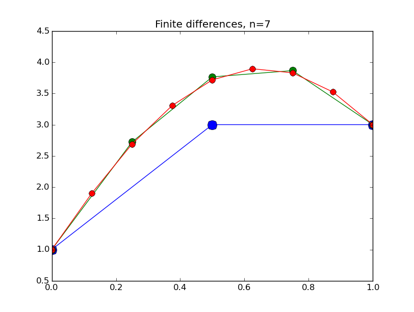
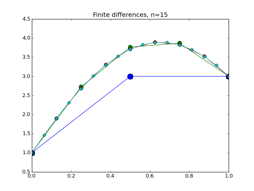
ODE boundary value problems
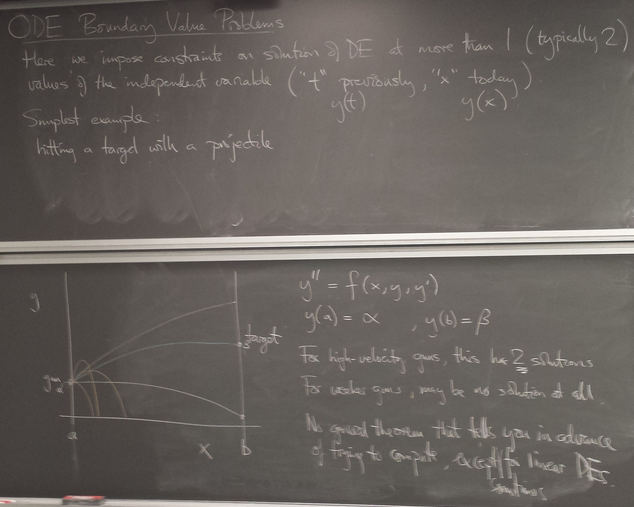
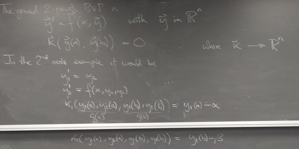
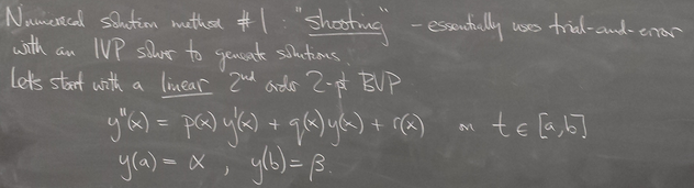
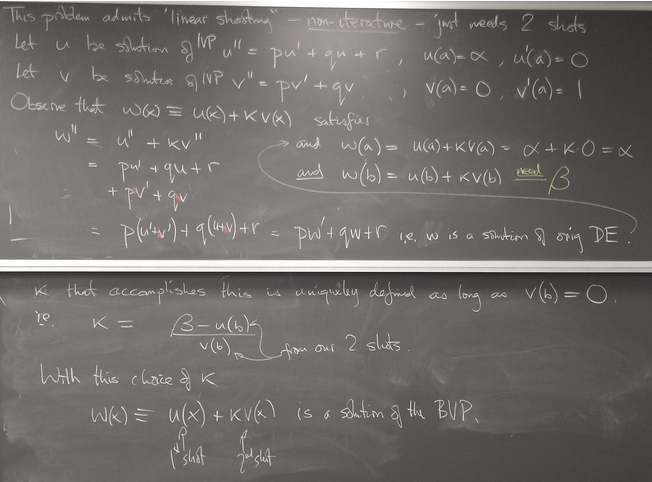
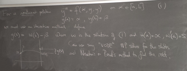
Method 2: Finite differences
Thursday, Feb 18, 2016
Concrete examples: linear problem
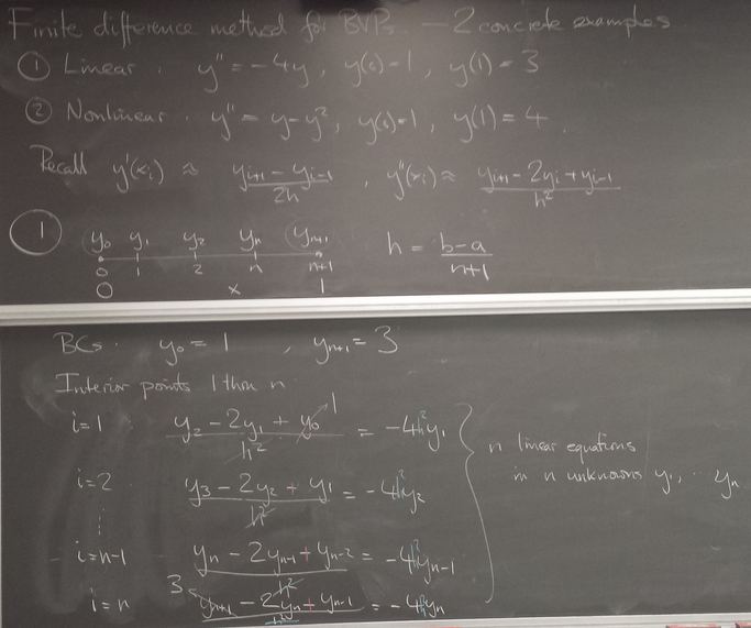
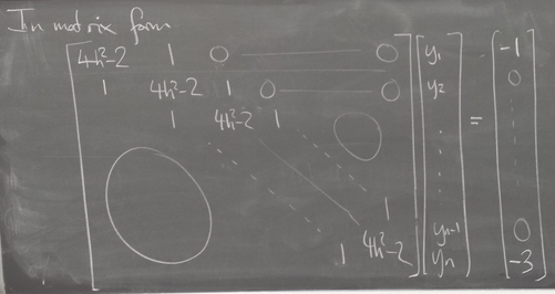
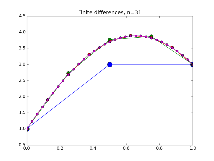
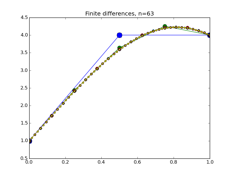
from numpy import *
from pylab import plot,show,ion,title,ylim,savefig
import sys

def prep_matrix(n):
        m = zeros((n,n))
        for i in range(n-1):
                m[i,i+1]=1.
                m[i+1,i]=1.
        return m

a = 0.; ya = 1.
b = 1.; yb = 3.
gamma = -4.  # coefficient on RHS of ODE


ion()
for k in range(1,7):

        n = 2**k-1

        m = prep_matrix(n)
        h = (b-a)/float(n+1)
        fill_diagonal(m,-gamma*h*h-2.)
        rhs = zeros(n)
        rhs[ 0] = -ya
        rhs[-1] = -yb
        print 'm'
        print m
        print 'rhs'
        print rhs
        y = linalg.solve(m,rhs)

        t = linspace(a,b,n+2)
        plot( t,hstack(( [ya],y,[yb] )) ,'o-',markersize=40./(k+2) )
        title("Finite differences, n="+str(n))
        ylim(0.5,4.5)
        savefig(sys.argv[0]+'_'+str(k).zfill(4)+'.png')
        raw_input("Hit Enter to continue")
Results:
Concrete examples: nonlinear problem
We wrote the following code in class, using the linear system code above as a starting point.
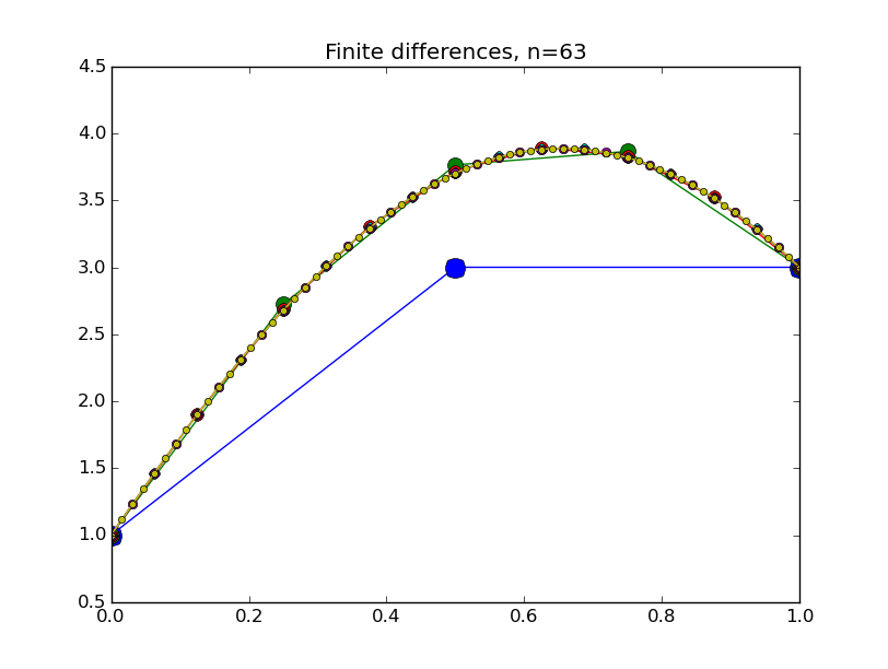
from numpy import *
from pylab import plot,show,ion,title,ylim,savefig
import sys

def prep_matrix(n):
        m = zeros((n,n))
        for i in range(n-1):
                m[i,i+1]=1.
                m[i+1,i]=1.
        return m

a = 0.; ya = 1.
b = 1.; yb = 4.

def myfdf(y,h,ya,yb):
        n = len(y)
        df = prep_matrix(n)
        fill_diagonal(df, -2. - h**2*(1.-2.*y) )
        f = -2.*y - h**2*(y-y**2)
        f[0]  += ya
        f[1:] += y[:-1]
        f[:-1]+= y[1:]
        f[-1] += yb
        return f,df

def newton(fdf,y0,tol,*args):
        y = array(y0)
        count = 0
        while True:
                f,df = fdf(y,*args)
                s = linalg.solve(df,-f)
                y += s
                count += 1
                if linalg.norm(s) < tol:
                        print 'Newton did',count,'iterations'
                        return y

ion()
for k in range(1,7):

        n = 2**k-1
        h = (b-a)/float(n+1)
        tol = 1.e-6

        y = linspace(ya,yb,n+2)[1:-1]  # guess is linear interpolant between ya and yb
        y = newton(myfdf,y,tol,h,ya,yb)

        t = linspace(a,b,n+2)
        plot( t,hstack(( [ya],y,[yb] )) ,'o-',markersize=40./(k+2) )
        title("Finite differences, n="+str(n))
        ylim(0.5,4.5)
        savefig(sys.argv[0]+'_'+str(k).zfill(4)+'.png')
        raw_input("Hit Enter to continue")
Results:
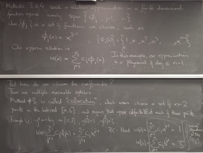
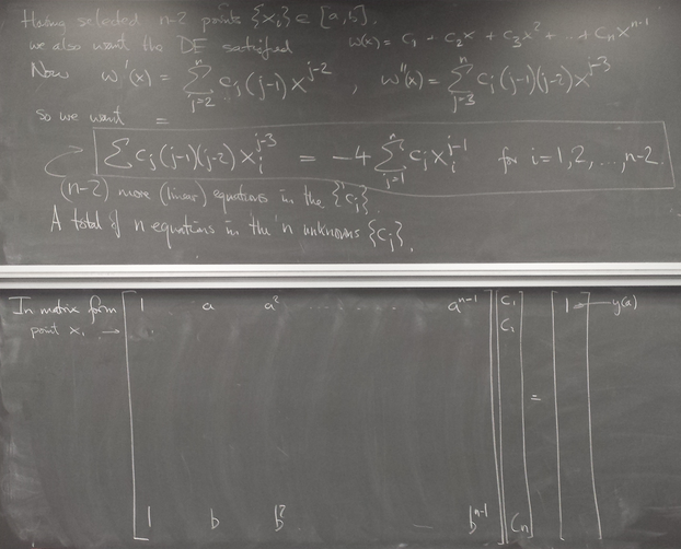
Collocation, cont'd
Implementing the collocation method (linear problem)
We wrote the following code from scratch in class:
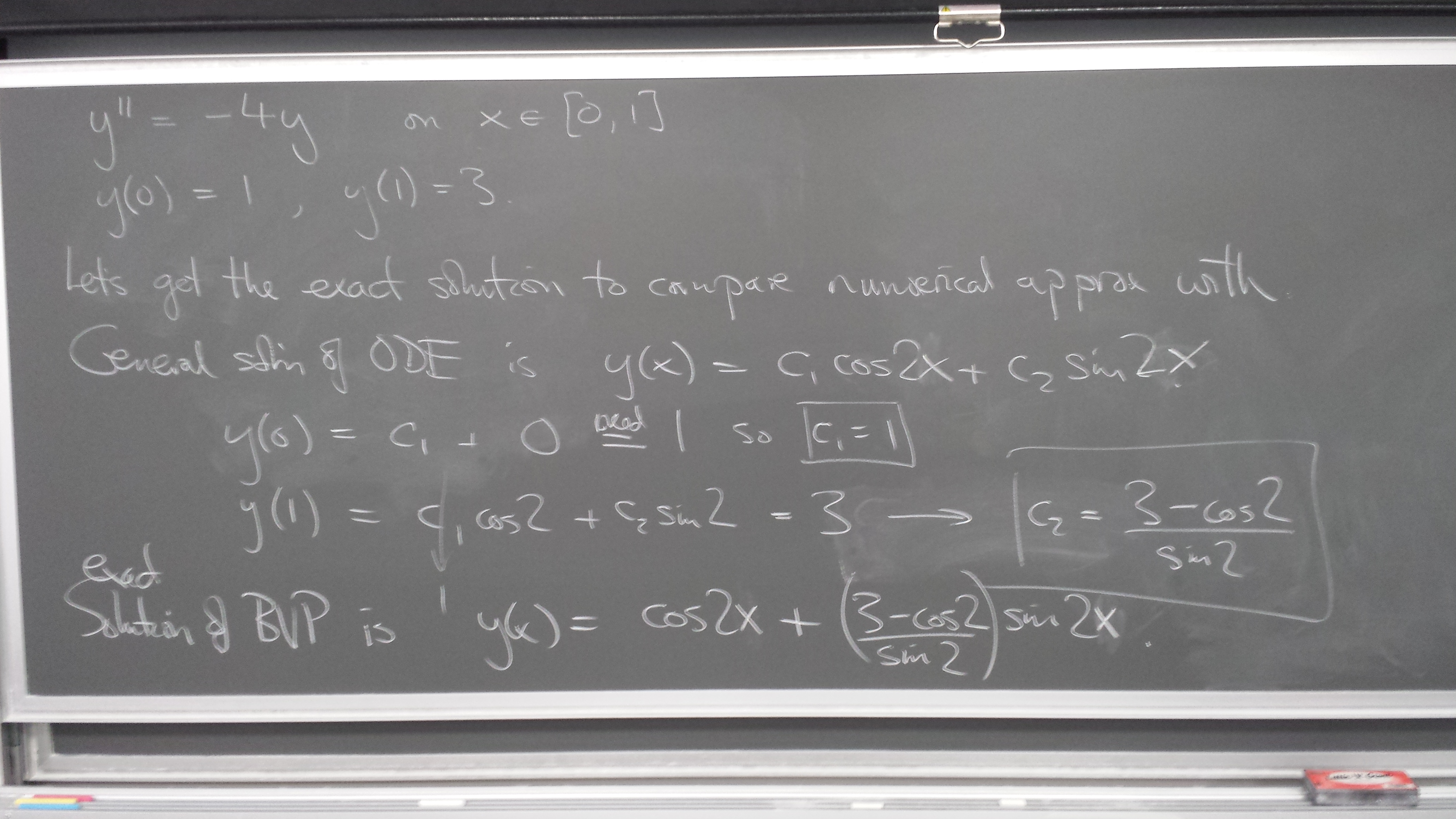
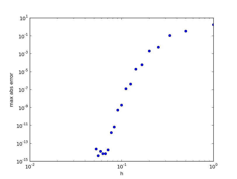
from numpy import *
import pylab as pl

def collocation_matrix(x,a,b,gamma):
      n = len(x)
      A = empty((n,n))

      for j in range(n): A[0  ,j] = a**j

      for i in range(1,n):
              for j in range(n):
                      A[i,j] = float(j)*float(j-1)*x[i]**(j-2) - gamma*x[i]**j  # differs from chalk
                                                       # due to 0-based indexing
      for j in range(n): A[n-1,j] = b**j

      return A

a = 0.; b = 1.
alpha = 1.; beta = 3.
gamma = -4.

def exact(x,gamma):
      assert gamma==-4.
      return cos(2*x) + (3.-cos(2.))/sin(2.)*sin(2*x)

for n in [4]: range(2,21):

      x = linspace(a,b,n)
      A = collocation_matrix(x,a,b,gamma)
      #print A
      rhs = zeros(n)
      rhs[  0] = alpha
      rhs[n-1] = beta

      c = linalg.solve(A,rhs)
      #print c

      # evaluate our approximate solution on a dense grid
      xx = linspace(a,b,500)
      w = zeros_like(xx)
      for j in range(n):
              w += c[j]*xx**j
      pl.subplot(211)
      pl.plot(xx,w,'r')
      pl.plot(xx,exact(xx,gamma),'b')
      pl.subplot(212)
      pl.plot(xx, w-exact(xx,gamma), 'g' )  # error
      pl.plot(xx, 0*xx, 'k' )  # error

      print n,abs(w-exact(xx,gamma)).max()

pl.show()
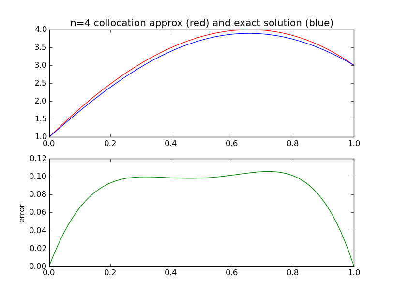
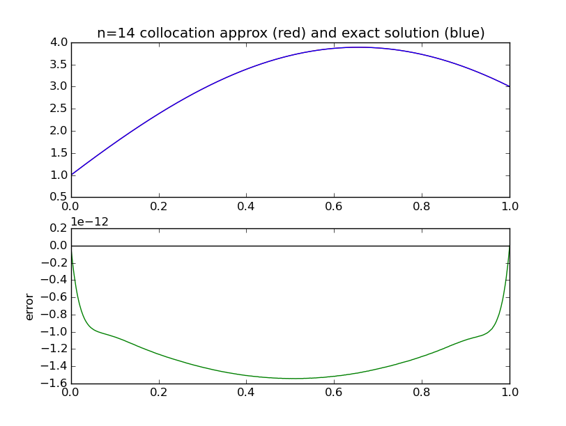
Comparison with exact solution
for n in range(2,21):
  ...
  print n,abs(w-exact(xx,gamma)).max()
n max abs error
2 1.70640053218
3 0.335398960028
4 0.105699361183
5 0.00528455009821
6 0.00196603344336
7 5.73185009491e-05
8 1.94053114497e-05
9 3.97602567981e-07
10 1.20731387554e-07
11 1.87477300351e-09
12 5.07189845678e-10
13 6.35114183467e-12
14 1.54454227186e-12
15 1.84297022088e-14
16 7.1054273576e-15
17 7.1054273576e-15
18 1.24344978758e-14
19 3.99680288865e-15
20 2.35367281221e-14
We see that the maximum error drops very rapidly to around machine epsilon for a very modest number of collocation points: n=16. There is nothing to be gained by increasing n beyond this.
Method 4: Galerkin method
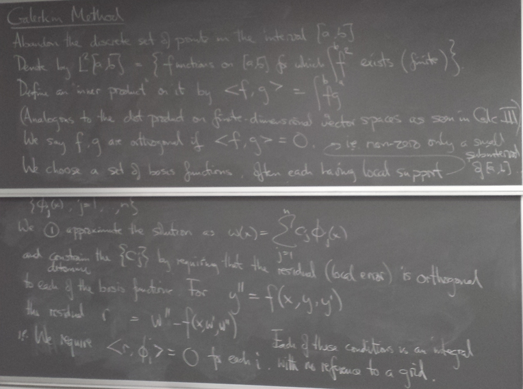
Implementation of Galerkin on linear problem
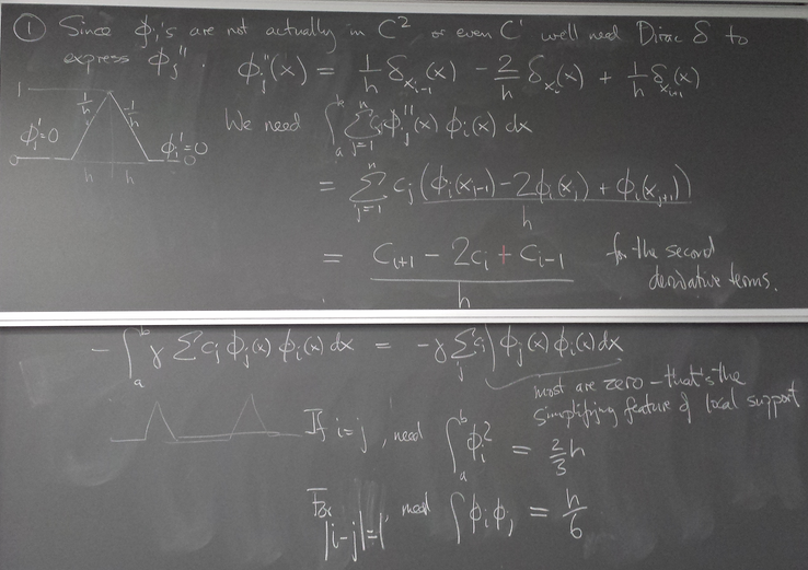
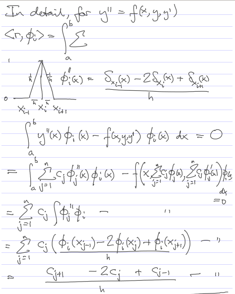
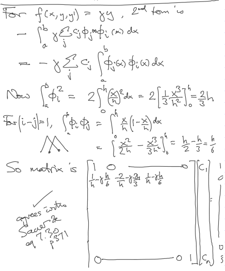
We fix c1 and cn by imposing the BCs, and require orthogonality of the residual only with phi_2 through phi_(n-1).
Partial Differential Equations
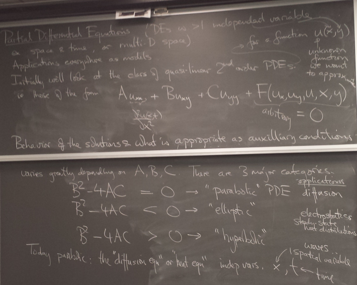
Parabolic PDEs: the heat equation
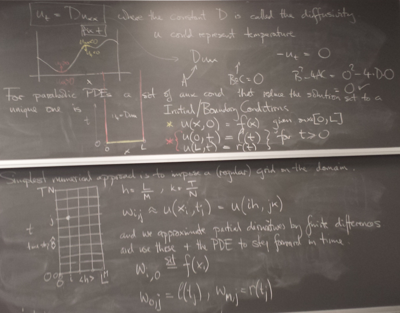
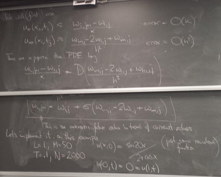
Forward difference method and instability
Here is the first version we wrote in class - the computation only:
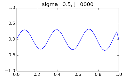
from numpy import *
import matplotlib.pyplot as pl

D = 4.
L = 1.
M = 50
T = .1
N = 2000

h = L/float(M)  # spatial grid spacing
k = T/float(N)  # time step

sigma = D*k/h**2

def f(x): return sin(20*x)/(2+cos(x))
def l(t): return 0.
def r(t): return 0.

x = linspace(0,L,M+1)

w = f(x)  # set initial values

for j in range(N):
      w[1:-1] += sigma*( w[:-2] - 2*w[1:-1] + w[2:]   )
      newt = k*(j+1)
      w[ 0] = l(newt)
      w[-1] = r(newt)

print w
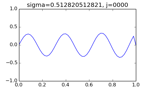
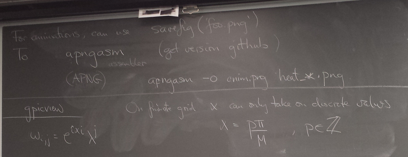
And here is the elaborated version that generated an animated plot. I added a "savefig" after class so that I could make an animated PNG (APNG) to embed in this webpage.
from numpy import *
import pylab as pl #matplotlib.pyplot as pl

D = 4.
L = 1.
M = 50
T = .1
N = 1950# 2000

h = L/float(M)  # spatial grid spacing
k = T/float(N)  # time step

sigma = D*k/h**2

def f(x): return sin(20*x)/(2+cos(x))
def l(t): return 0.
def r(t): return 0.

x = linspace(0,L,M+1)

w = f(x)  # set initial values

pl.figure(figsize=(5,3)) # added after class
pl.ion()
pl.plot([0,L],[-1,1],'w' )  # invisible line to set plot scale
p, = pl.plot(x,w,'b')

for j in range(N):
      print j
      w[1:-1] += sigma*( w[:-2] - 2*w[1:-1] + w[2:]   )
      newt = k*(j+1)
      w[ 0] = l(newt)
      w[-1] = r(newt)
      p.set_ydata(w)  # update the curve in the plot
      pl.title('sigma='+str(sigma)+', j='+str(j).zfill(4))
      pl.draw()

      if j%5==0: pl.savefig('heat_'+str(j).zfill(4)+'.png') # added after class
      if abs(w).max()>10.: break                            # added after class
print w

pl.ioff()
pl.show()
Results with two slightly different time steps:
Thursday, March 3, 2016
Methods for parabolic PDE, cont'd
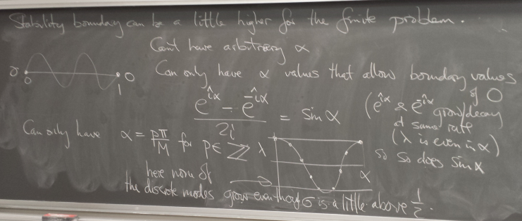
Homogeneous Dirichlet BCs: sin basis
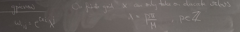
Of all the functions sin(αx), with α = pπ ⁄ L and p ∈ ℤ, only M − 1 of them are non-zero and distinct on the grid xi = iL ⁄ M, i ∈ 0, 1, 2, ..., M. In the case of M = 10 illustrated below, there are 9 non-trivial functions on the grid. Each of these is an eigenfunction of our time-stepping operator.
Discrete sines as a basis for ℝM − 1 = ℝ9:
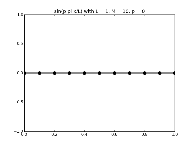
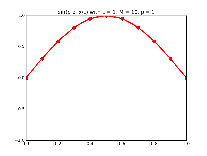
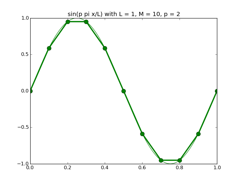
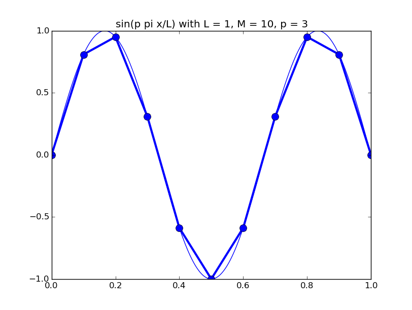
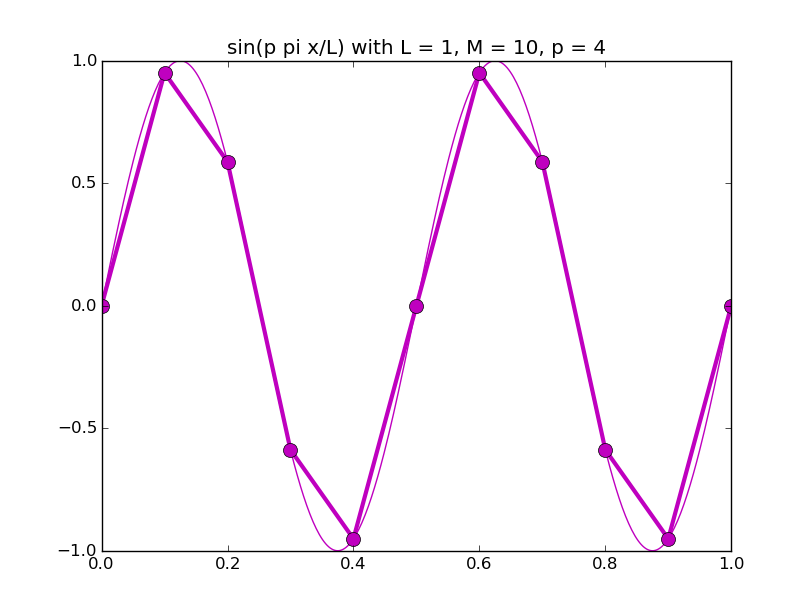
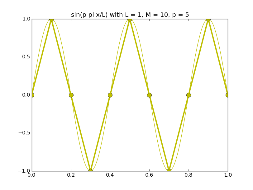
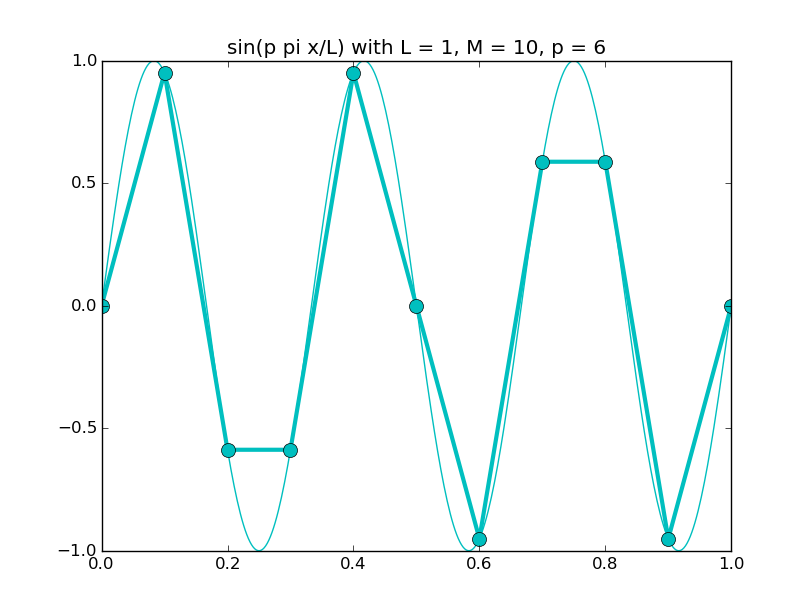
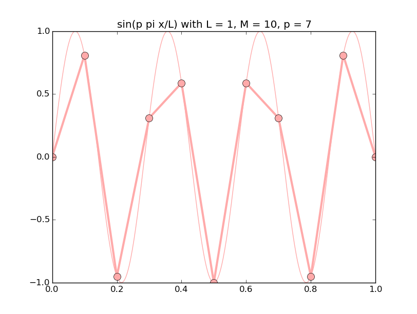
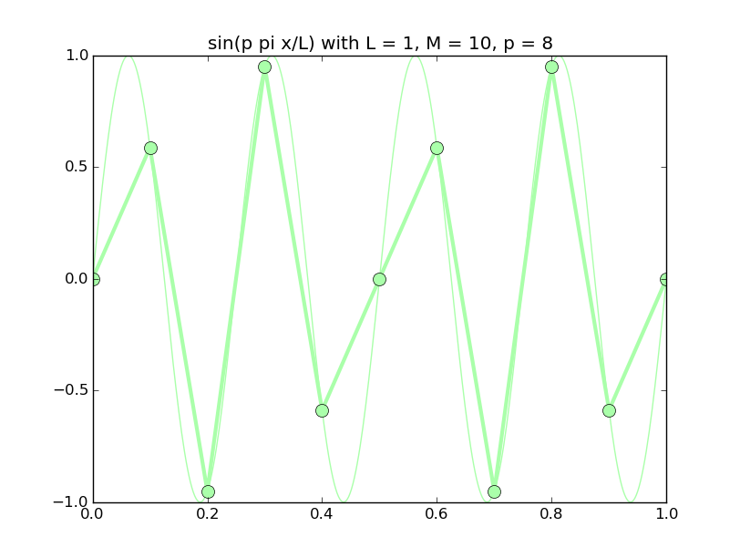
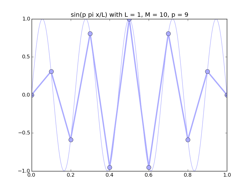
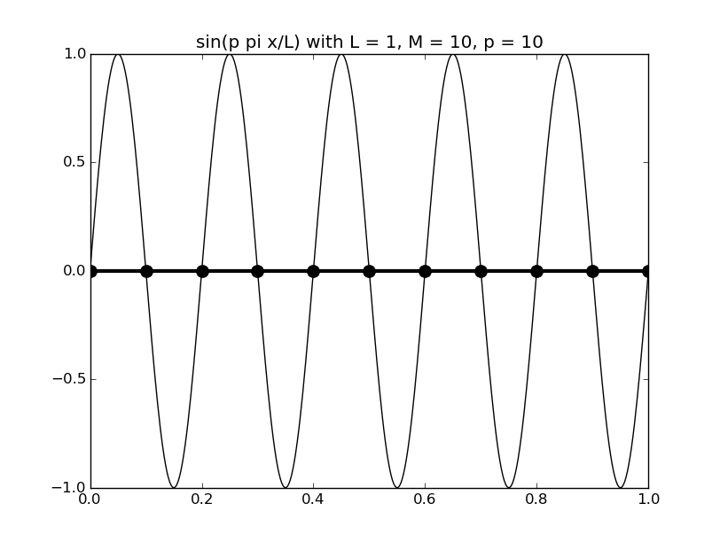
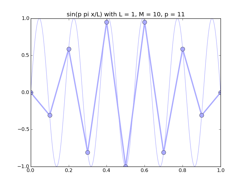
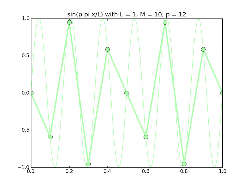
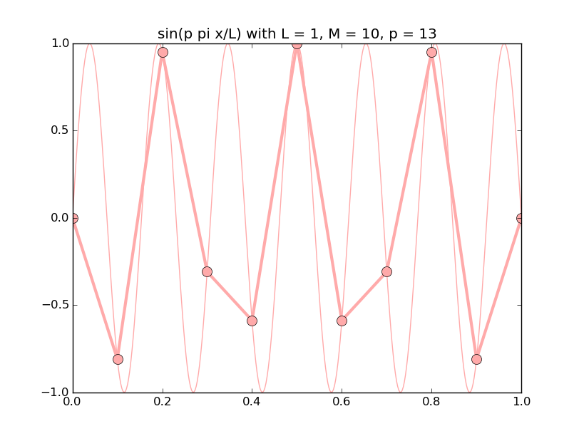
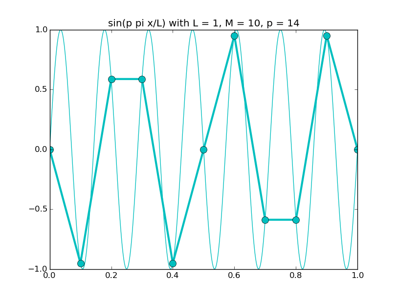
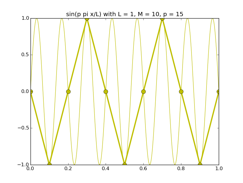
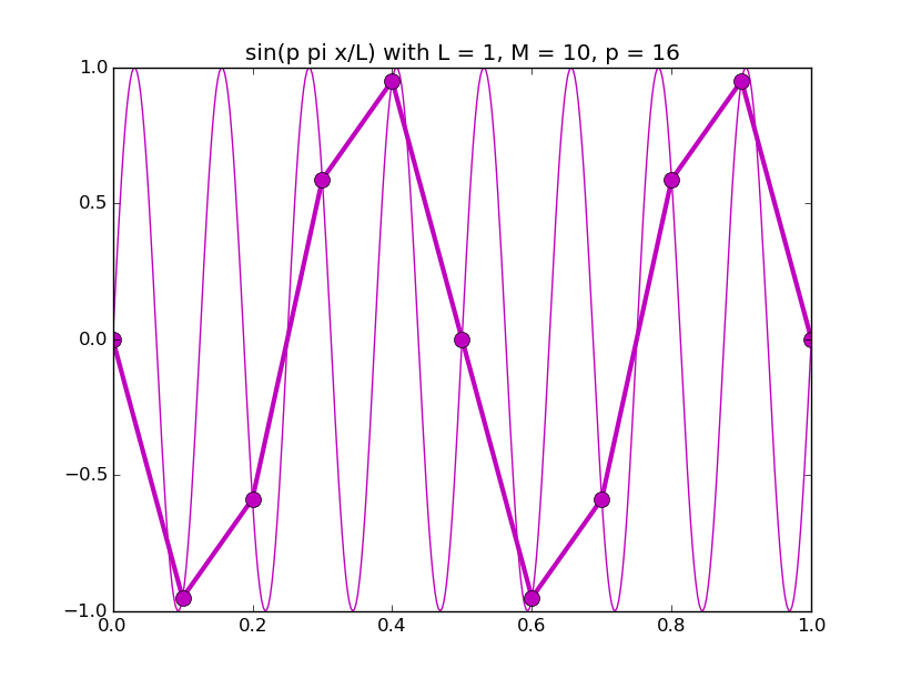
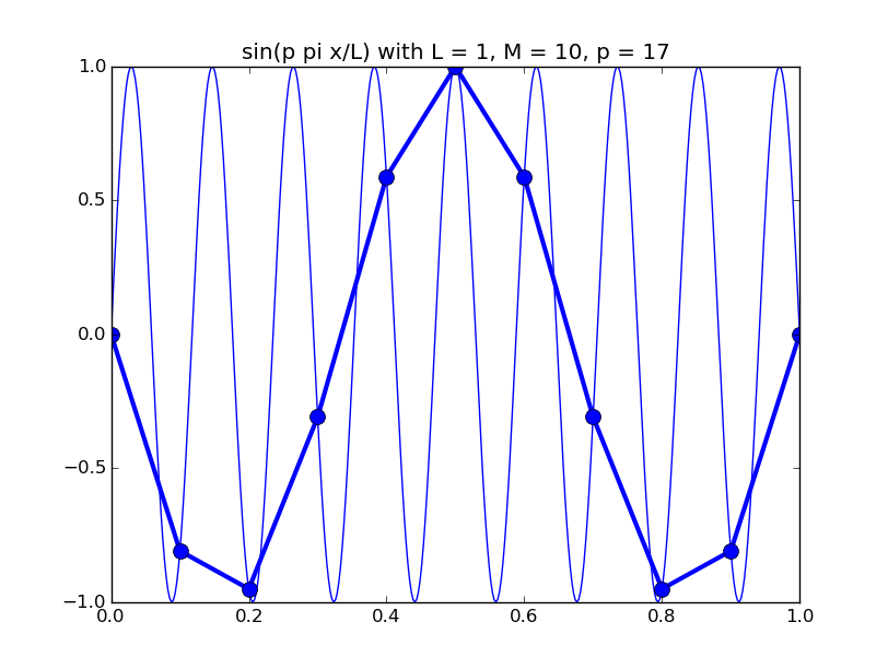
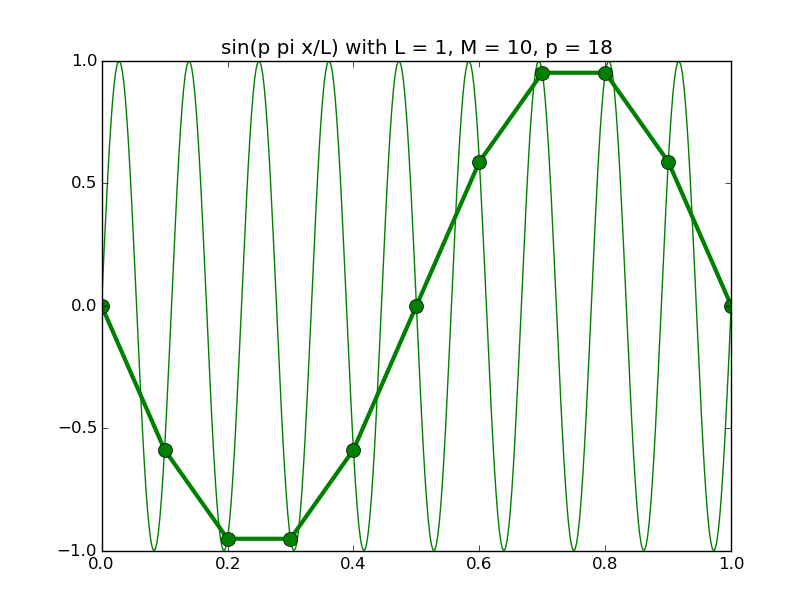
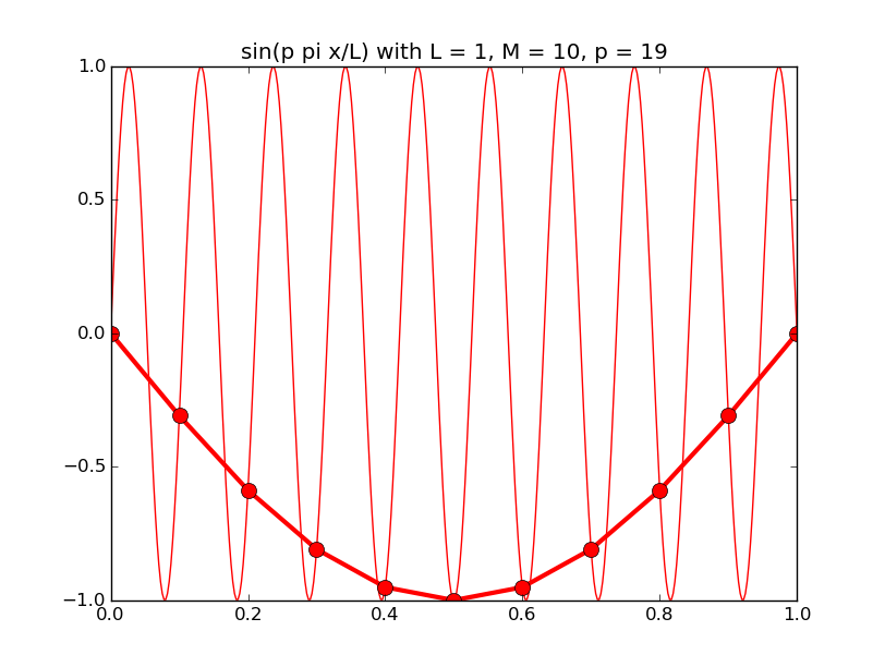
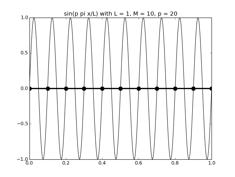
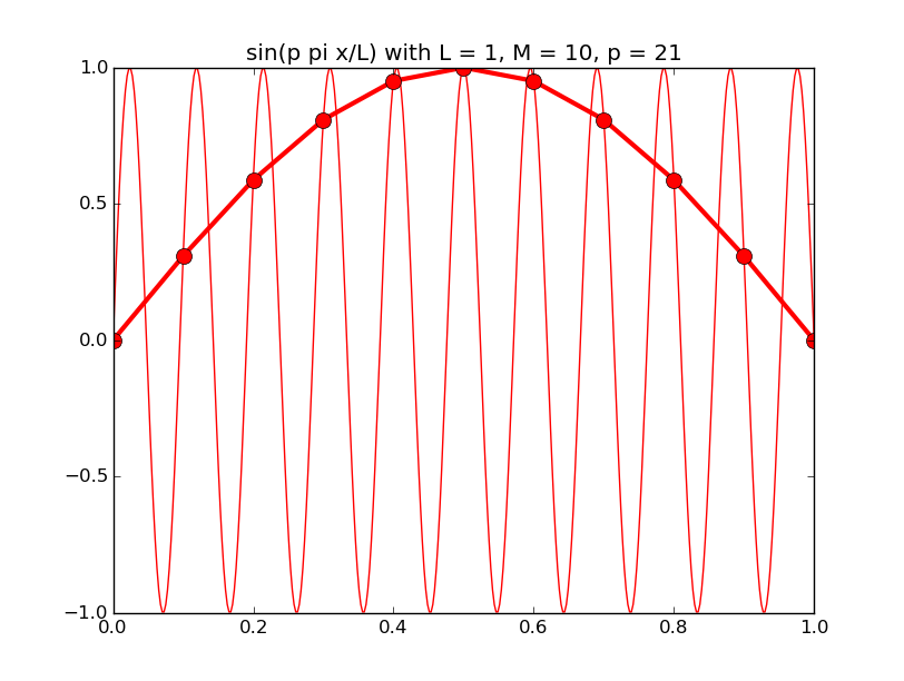
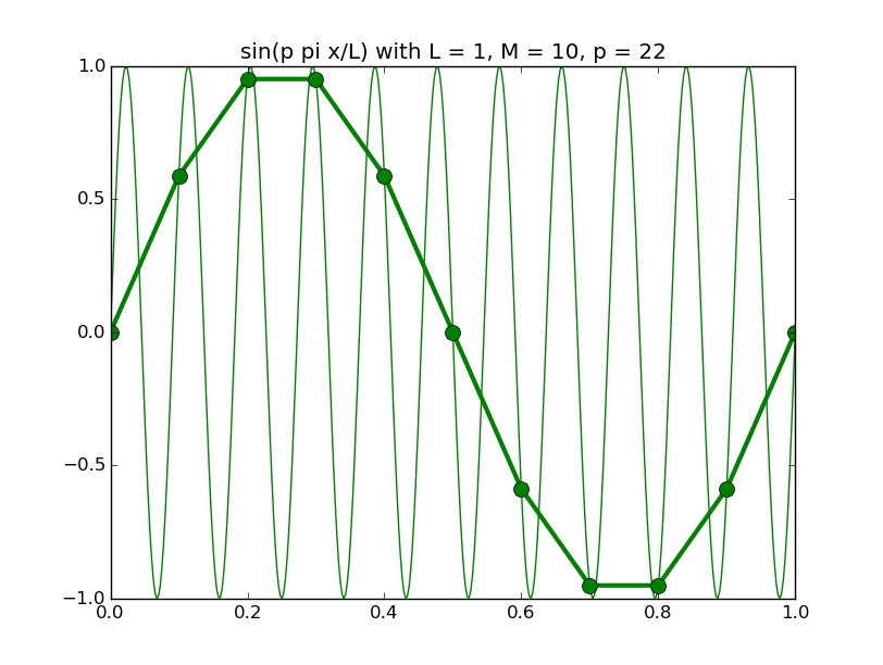
The above pictures generated by discrete_sines.py.
Unconditionally stable methods: backwards differentiation scheme
Because the stability limit of the previous method means that increasing the spatial resolution by a factor of 10 requires 1000 times as much computational work, we are interested in methods that do not have this restriction.
One such method is to use an approximation to uxx at the forward time.
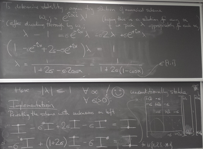
We wrote the following code in class (using the code for the Forward Difference Scheme as a starting point)
from numpy import *
import matplotlib.pyplot as pl

D = 4.
L = 1.
M = 50 #5 #
T = .1
N = 200 # 1950# 2000

h = L/float(M)  # spatial grid spacing
k = T/float(N)  # time step

sigma = D*k/h**2

def f(x): return sin(20*x)/(2+cos(x))
def l(t): return 0.
def r(t): return 0.

x = linspace(0,L,M+1)

w = f(x)  # set initial values

A = zeros((M-1,M-1))
fill_diagonal(A,1.+2.*sigma)     # diagonal
fill_diagonal(A[1:,:-1],-sigma)  # subdiagonal
fill_diagonal(A[:-1,1:],-sigma)  # superdiagonal

#print A

pl.ion()
pl.plot([0,L],[-1,1],'w' )  # invisible line to set plot scale
p, = pl.plot(x,w,'b')

for j in range(N):
        # first update the boundary values
        newt = k*(j+1)
        w[ 0] = l(newt)
        w[-1] = r(newt)
        rhs = array(w[1:-1])
        rhs[ 0] += sigma*w[ 0]
        rhs[-1] += sigma*w[-1]
        w[1:-1] = linalg.solve(A,rhs)

        p.set_ydata(w)  # update the curve in the plot
        pl.title('j='+str(j).zfill(4))
        pl.draw()
print w

pl.ioff()
pl.show()
We see the method is stable even for time step 10 times bigger than the Forward Difference Scheme would allow.
Tridiagonal solver
It is wasteful to use a full-system solver on this tridiagonal linear system. Here is a version of the code where I've modified it to use scipy.linalg.solve_banded():
from numpy import *
import matplotlib.pyplot as pl
from scipy.linalg import solve_banded  ###########

D = 4.
L = 1.
M = 50 #5 #
T = .01
N = 20

h = L/float(M)  # spatial grid spacing
k = T/float(N)  # time step

sigma = D*k/h**2

def f(x): return sin(20*x)/(2+cos(x))
def l(t): return 0.
def r(t): return 0.

x = linspace(0,L,M+1)

w = f(x)  # set initial values

A = zeros((3,M-1))  # just make space for the 3 diagonals
A[0,1:] = -sigma       # subdiagonal
A[1,:  ] = 1.+2.*sigma  # diagonal
A[2,:-1] = -sigma       # superdiagonal

#print A

pl.ion()
pl.plot([0,L],[-1,1],'w' )  # invisible line to set plot scale
p, = pl.plot(x,w,'b')

for j in range(N):
        # first update the boundary values
        newt = k*(j+1)
        w[ 0] = l(newt)
        w[-1] = r(newt)
        rhs = array(w[1:-1])
        rhs[ 0] += sigma*w[ 0]
        rhs[-1] += sigma*w[-1]
        w[1:-1] = solve_banded( (1,1), A, rhs )

        p.set_ydata(w)  # update the curve in the plot
        pl.title('j='+str(j).zfill(4))
        pl.draw()
print w

pl.ioff()
pl.show()
Below we see the two versions give the same results, but the second one is more efficient.
$ py heat_bds.py
[  0.00000000e+00  -2.49165236e-05  -5.08192357e-05  -7.86792847e-05
  -1.09441681e-04  -1.44021373e-04  -1.83308417e-04  -2.28182491e-04
  -2.79535137e-04  -3.38296508e-04  -4.05462136e-04  -4.82114631e-04
  -5.69435343e-04  -6.68701801e-04  -7.81268167e-04  -9.08527677e-04
  -1.05185795e-03  -1.21255169e-03  -1.39173677e-03  -1.59029010e-03
  -1.80875030e-03  -2.04723318e-03  -2.30535344e-03  -2.58215492e-03
  -2.87605030e-03  -3.18477080e-03  -3.50532586e-03  -3.83397312e-03
  -4.16620017e-03  -4.49672055e-03  -4.81948838e-03  -5.12773724e-03
  -5.41404988e-03  -5.67046581e-03  -5.88863249e-03  -6.06000413e-03
  -6.17608879e-03  -6.22874027e-03  -6.21048656e-03  -6.11488179e-03
  -5.93686404e-03  -5.67309800e-03  -5.32227935e-03  -4.88537753e-03
  -4.36579530e-03  -3.76942749e-03  -3.10460680e-03  -2.38193158e-03
  -1.61397843e-03  -8.14910505e-04   0.00000000e+00]
$ py heat_bds_banded.py
[  0.00000000e+00  -2.49165236e-05  -5.08192357e-05  -7.86792847e-05
  -1.09441681e-04  -1.44021373e-04  -1.83308417e-04  -2.28182491e-04
  -2.79535137e-04  -3.38296508e-04  -4.05462136e-04  -4.82114631e-04
  -5.69435343e-04  -6.68701801e-04  -7.81268167e-04  -9.08527677e-04
  -1.05185795e-03  -1.21255169e-03  -1.39173677e-03  -1.59029010e-03
  -1.80875030e-03  -2.04723318e-03  -2.30535344e-03  -2.58215492e-03
  -2.87605030e-03  -3.18477080e-03  -3.50532586e-03  -3.83397312e-03
  -4.16620017e-03  -4.49672055e-03  -4.81948838e-03  -5.12773724e-03
  -5.41404988e-03  -5.67046581e-03  -5.88863249e-03  -6.06000413e-03
  -6.17608879e-03  -6.22874027e-03  -6.21048656e-03  -6.11488179e-03
  -5.93686404e-03  -5.67309800e-03  -5.32227935e-03  -4.88537753e-03
  -4.36579530e-03  -3.76942749e-03  -3.10460680e-03  -2.38193158e-03
  -1.61397843e-03  -8.14910505e-04   0.00000000e+00]
$
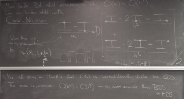
Unconditionally stable methods: Crank-Nicolson
An even better alternative is Crank-Nicolson, which is also unconditionally stable, and is moreover 2nd-order accurate in time as well as in space.
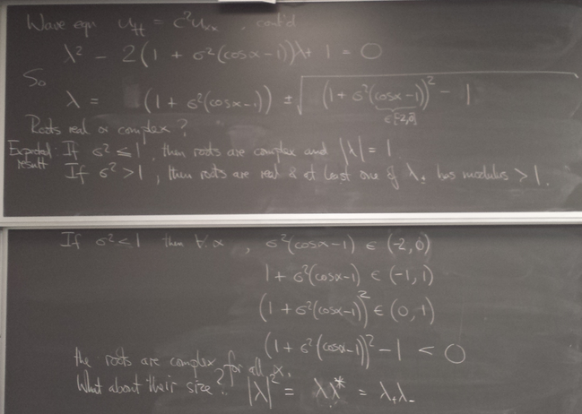
Finite difference method for hyperbolic PDE
We now turn to hyperbolic PDEs. The prototype is the "wave equation":

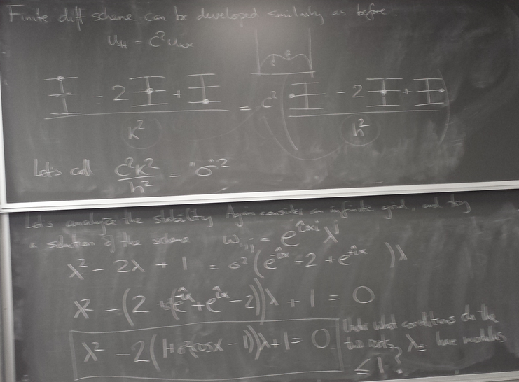
Tuesday, March 8, 2016
Start-up
You will implement this method in the homework.
Here is an animation I made of solving the wave equation in this way using a σ value that is just a little above the CFL limit: blow-up ensues!

wave_instability_demo.py shows the approximation to the solution for an initially undisplaced and stationary system and the boundary conditions give a little time-localized jiggle on the left.
Finite difference method for elliptic PDE
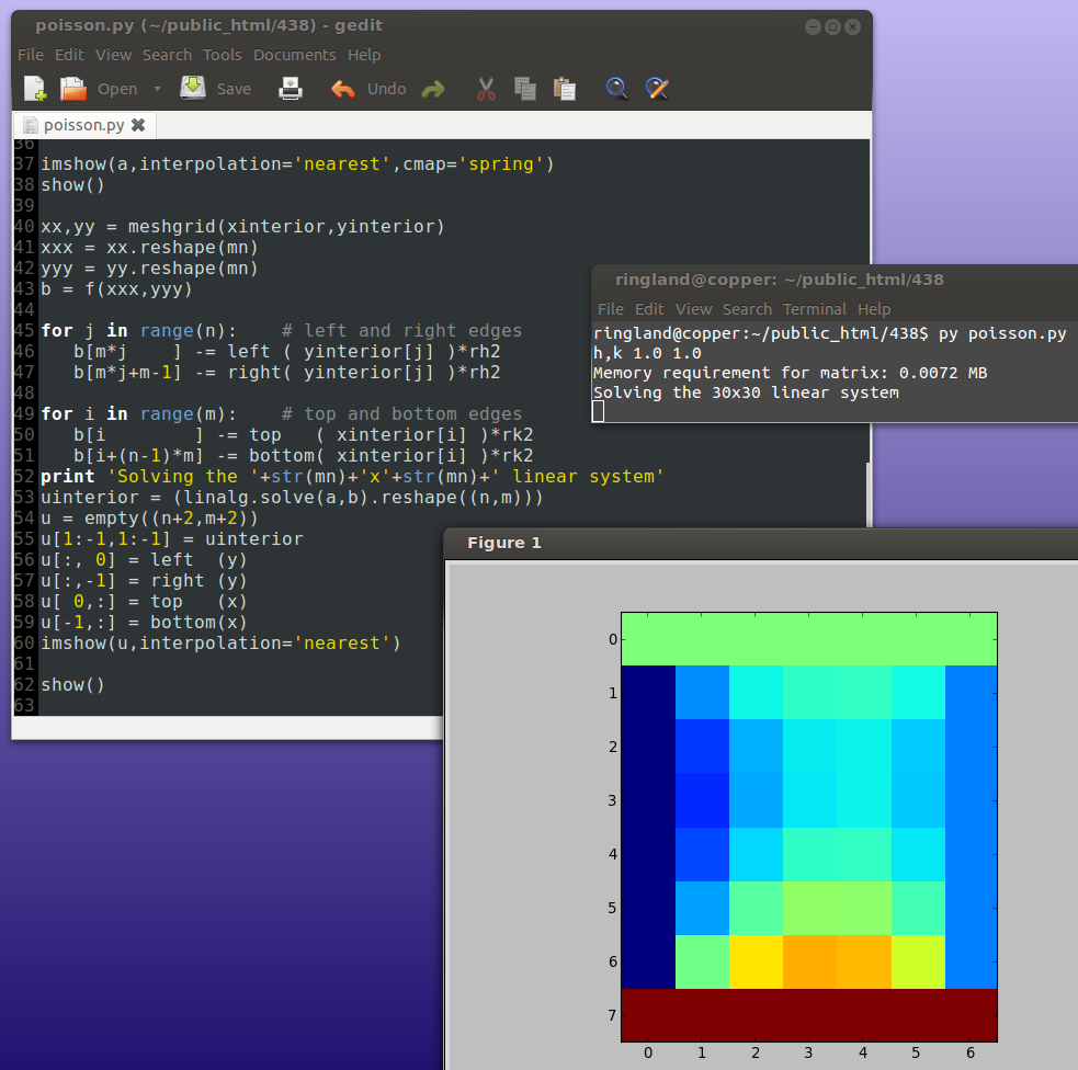
Prototype: Laplace/Poisson equation
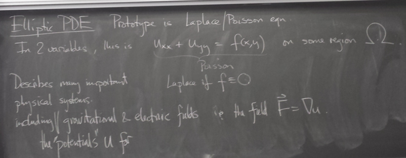
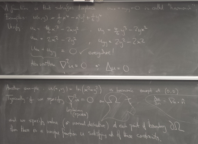
Harmonic functions: examples
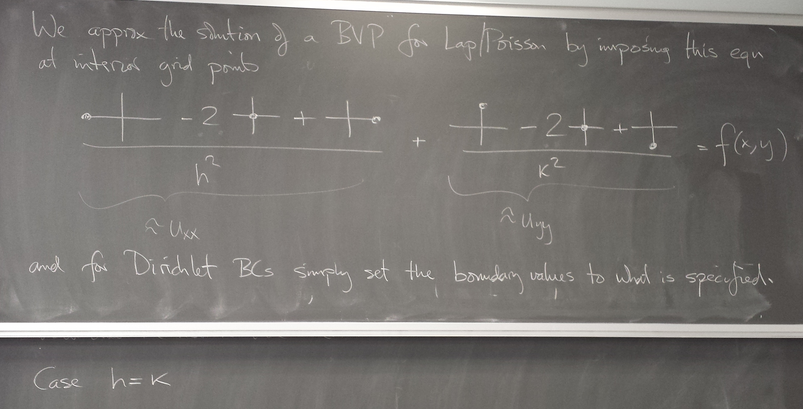
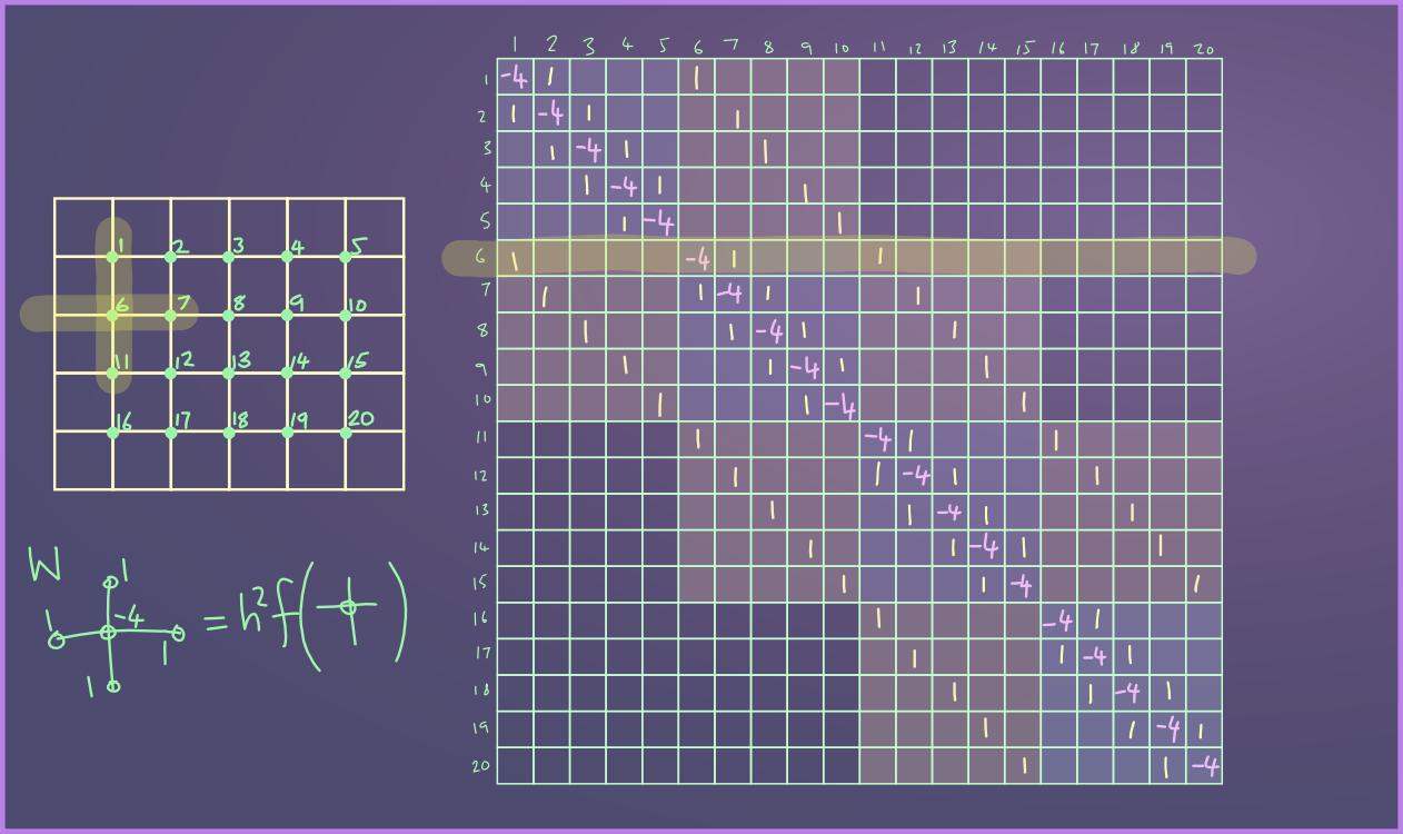
Implementation
Originally skipped.
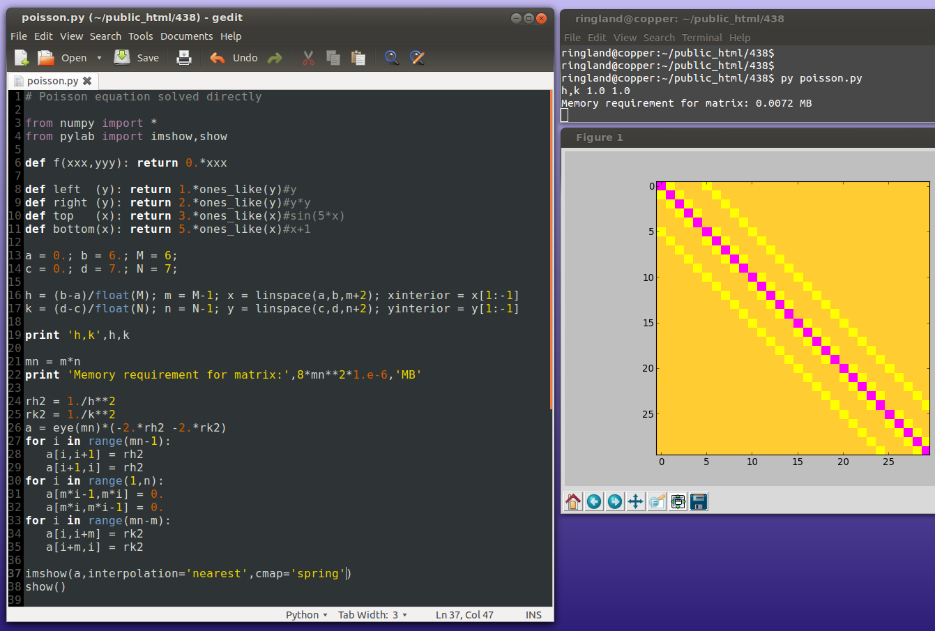
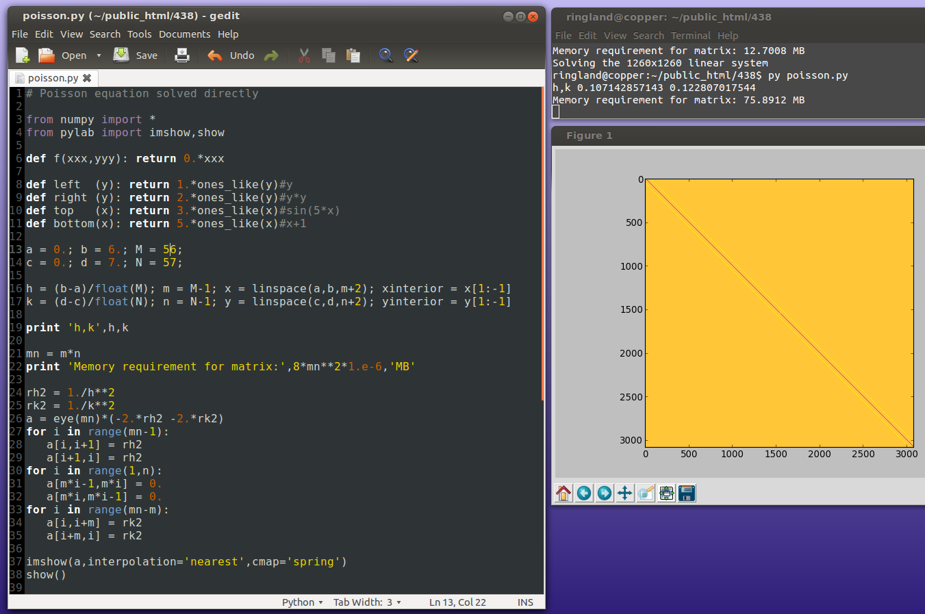
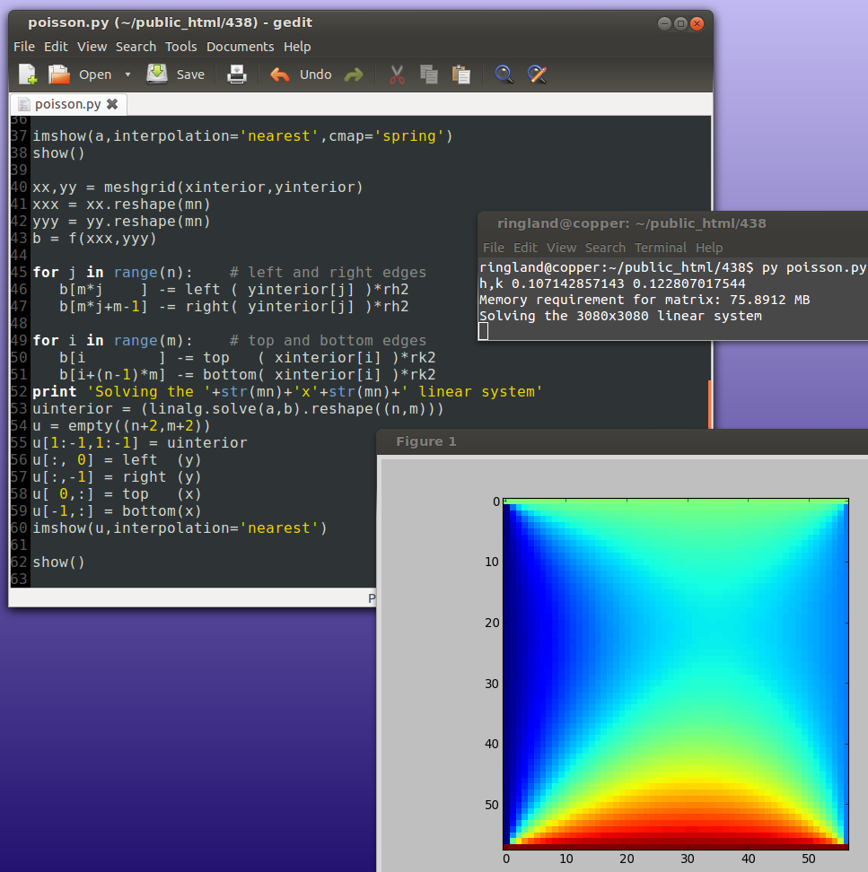
Because of the extreme sparsity of the matrix, the above is a very wasteful way of solving the system. Iterative methods are more efficient.
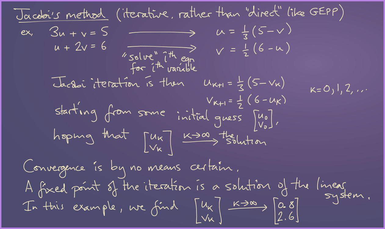
Iterative methods for sparse linear systems
Jacobi iteration
Thursday, March 10, 2016
Let's try it on the above example!
from numpy import *

def jacobi1(x):
        u,v= x
        return array([(5.-v)/3.,(6.-u)/2.])

x = array([1.,1.])
print x
for i in range(30):
        x = jacobi1(x)
        print x
[ 1.  1.]
[ 1.33333333  2.5       ]
[ 0.83333333  2.33333333]
[ 0.88888889  2.58333333]
[ 0.80555556  2.55555556]
[ 0.81481481  2.59722222]
[ 0.80092593  2.59259259]
[ 0.80246914  2.59953704]
[ 0.80015432  2.59876543]
[ 0.80041152  2.59992284]
[ 0.80002572  2.59979424]
[ 0.80006859  2.59998714]
[ 0.80000429  2.59996571]
[ 0.80001143  2.59999786]
[ 0.80000071  2.59999428]
[ 0.80000191  2.59999964]
[ 0.80000012  2.59999905]
[ 0.80000032  2.59999994]
[ 0.80000002  2.59999984]
[ 0.80000005  2.59999999]
[ 0.8         2.59999997]
[ 0.80000001  2.6       ]
[ 0.8  2.6]
[ 0.8  2.6]
[ 0.8  2.6]
[ 0.8  2.6]
[ 0.8  2.6]
[ 0.8  2.6]
[ 0.8  2.6]
[ 0.8  2.6]
[ 0.8  2.6]
Converged to the solution!
What if we try it with the equations in the other order (a mathematically equivalent system):
def jacobi2(x):
        u,v= x
        return array([6.-2.*v, 5. - 3.*u])
[ 1.  1.]
[ 4.  2.]
[ 2. -7.]
[ 20.  -1.]
[  8. -55.]
[ 116.  -19.]
[  44. -343.]
[ 692. -127.]
[  260. -2071.]
[ 4148.  -775.]
[  1556. -12439.]
[ 24884.  -4663.]
[  9332. -74647.]
[ 149300.  -27991.]
[  55988. -447895.]
[ 895796. -167959.]
[  335924. -2687383.]
[ 5374772. -1007767.]
[  2015540. -16124311.]
[ 32248628.  -6046615.]
[ 12093236. -96745879.]
[  1.93491764e+08  -3.62797030e+07]
[  7.25594120e+07  -5.80475287e+08]
[  1.16095058e+09  -2.17678231e+08]
[  4.35356468e+08  -3.48285174e+09]
[  6.96570348e+09  -1.30606940e+09]
[  2.61213880e+09  -2.08971104e+10]
[  4.17942209e+10  -7.83641641e+09]
[  1.56728328e+10  -1.25382663e+11]
[  2.50765325e+11  -4.70184985e+10]
[  9.40369969e+10  -7.52295975e+11]
Spectacularly fails to converge! What is going on?
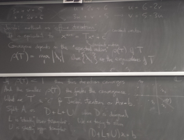
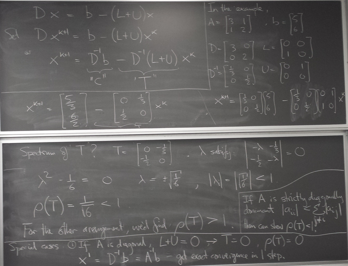
For matrices we encounter in solving elliptic PDEs, it does converge.
Jacobi iteration for Laplace on rectangle
Solve Laplace on rectangle with square grid (x-spacing and y-spacing the same).
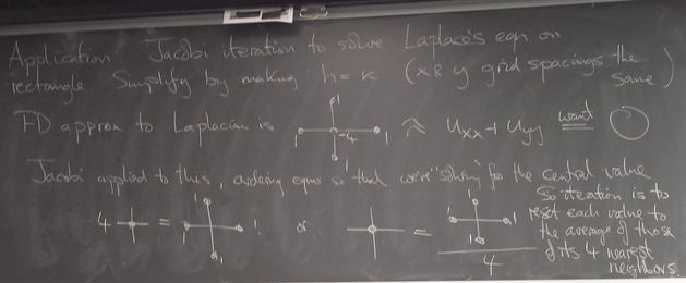
Let's redo that manual computation by computer:
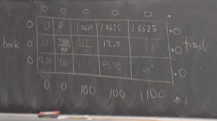
from numpy import *
from pylab import *

set_printoptions(linewidth=200)
M = 4
N = 6

w = zeros((M+1,N+1))

# BCs
w[-1,-4:-1] = 100.
print w
print

for k in range(3):
        w[1:-1,1:-1] = 0.25*(w[0:-2,1:-1]+ w[2:,1:-1] + w[1:-1,0:-2]+ w[1:-1,2:])
        print w
        print
$ py jacobi_laplace_small.py

[[   0.    0.    0.    0.    0.    0.    0.]
 [   0.    0.    0.    0.    0.    0.    0.]
 [   0.    0.    0.    0.    0.    0.    0.]
 [   0.    0.    0.    0.    0.    0.    0.]
 [   0.    0.    0.  100.  100.  100.    0.]]

[[   0.    0.    0.    0.    0.    0.    0.]
 [   0.    0.    0.    0.    0.    0.    0.]
 [   0.    0.    0.    0.    0.    0.    0.]
 [   0.    0.    0.   25.   25.   25.    0.]
 [   0.    0.    0.  100.  100.  100.    0.]]

[[   0.      0.      0.      0.      0.      0.      0.  ]
 [   0.      0.      0.      0.      0.      0.      0.  ]
 [   0.      0.      0.      6.25    6.25    6.25    0.  ]
 [   0.      0.      6.25   31.25   37.5    31.25    0.  ]
 [   0.      0.      0.    100.    100.    100.      0.  ]]

[[   0.        0.        0.        0.        0.        0.        0.    ]
 [   0.        0.        0.        1.5625    1.5625    1.5625    0.    ]
 [   0.        0.        3.125     9.375    12.5       9.375     0.    ]
 [   0.        1.5625    7.8125   37.5      42.1875   35.9375    0.    ]
 [   0.        0.        0.      100.      100.      100.        0.    ]]
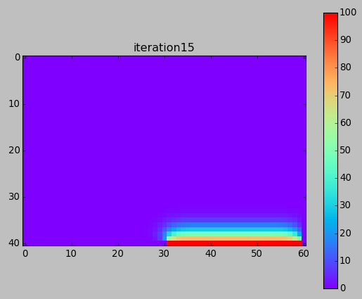
But with a higher resolution (more grid points), convergence is very slow:
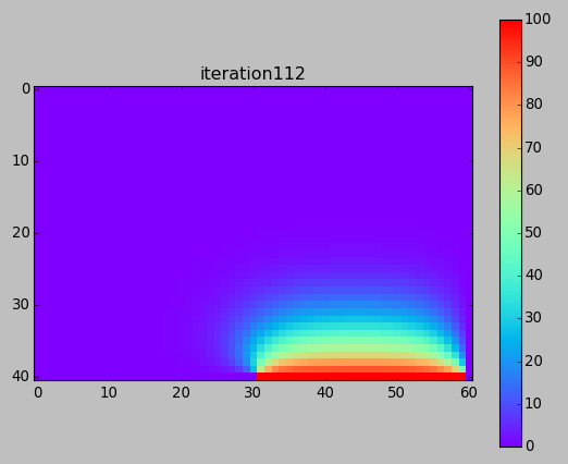
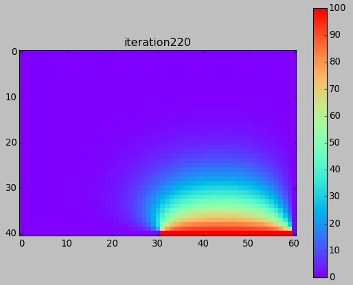
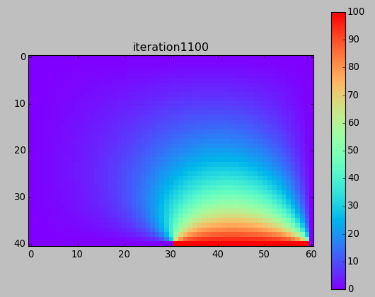
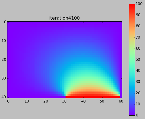
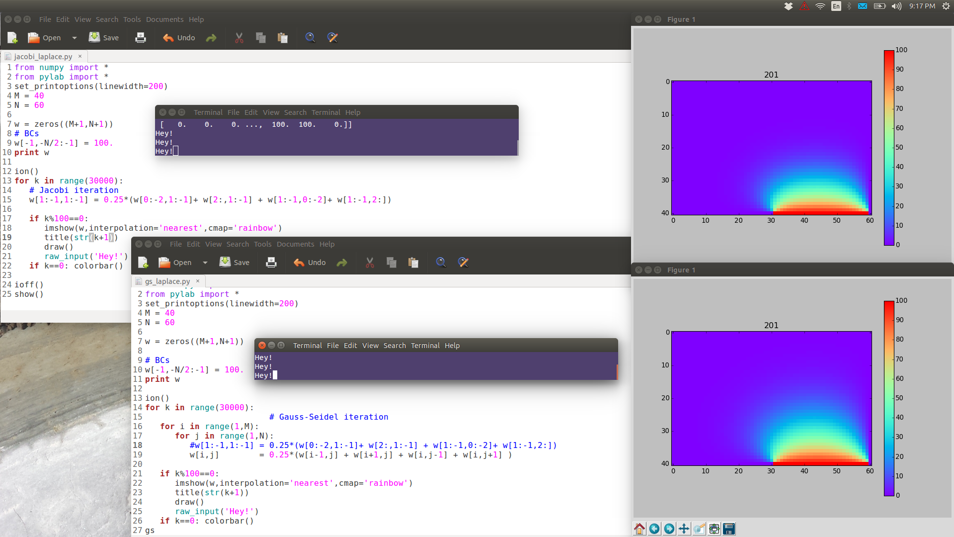
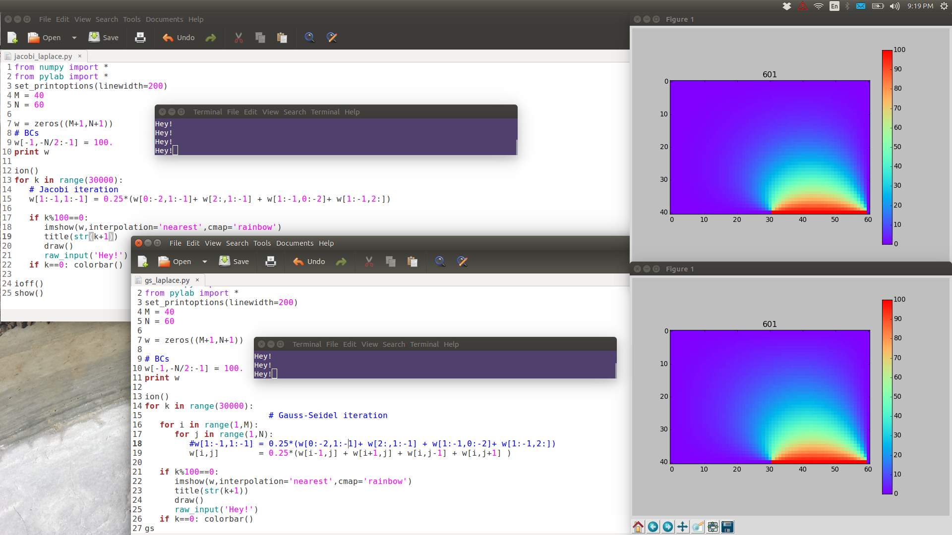
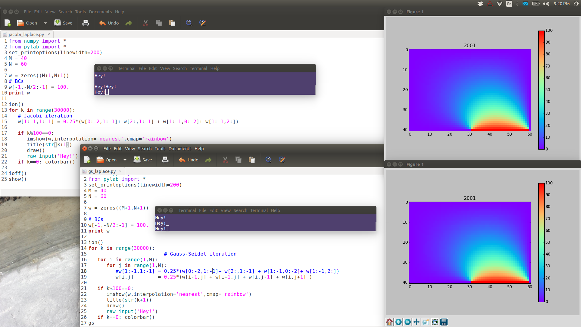
from numpy import *
from pylab import *

set_printoptions(linewidth=200)
M = 40
N = 60

w = zeros((M+1,N+1))

# BCs
w[-1,-N/2:-1] = 100.
print w

ion()
for k in range(30000):

        # computation
        w[1:-1,1:-1] = 0.25*(w[0:-2,1:-1]+ w[2:,1:-1] + w[1:-1,0:-2]+ w[1:-1,2:])

        # picture
        if k%100==0:
                imshow(w,interpolation='nearest',cmap='rainbow')
                title('iteration'+str(k))
                draw()
        if k==0: colorbar()

ioff()
show()
Next time (after Spring Break) ...
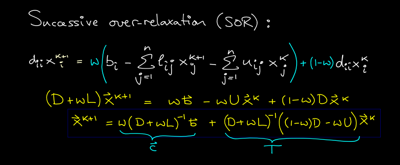
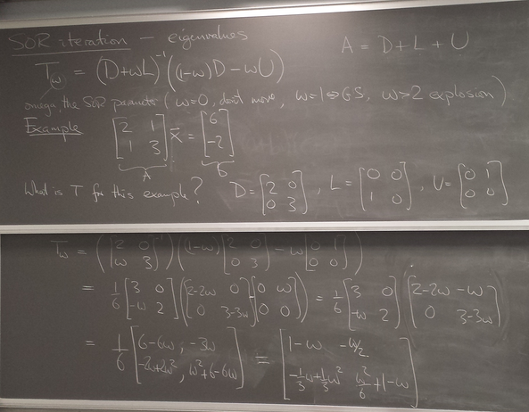
Successive Over-Relaxation
SOR (Java) demo
I wrote this Java demo some years ago. It uses Java features that are now deprecated/not working. So no click responses. Need to recompile (javac) to change w value.
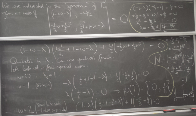
Eigenvalues of the iteration
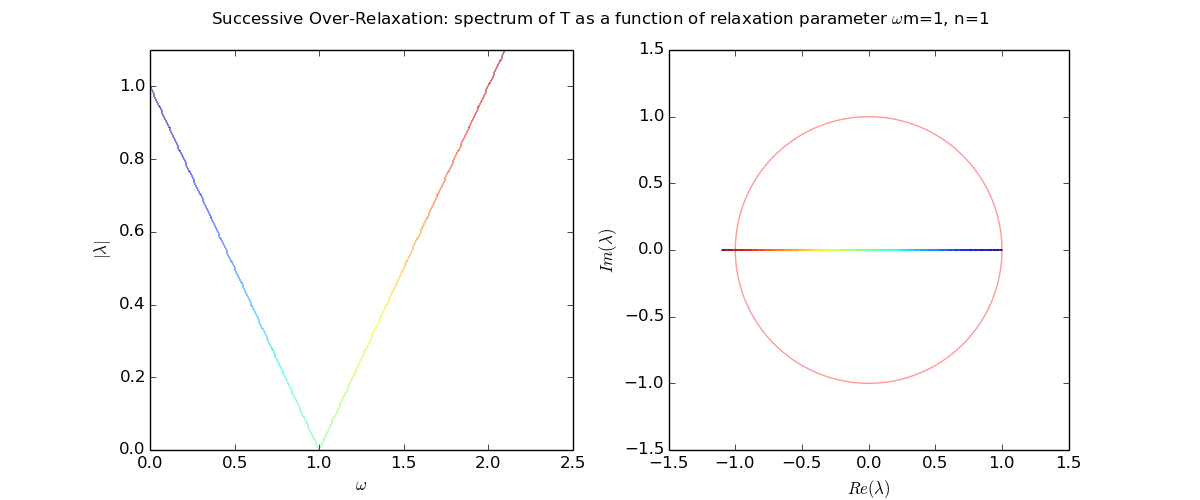
Eigenvalues as a function of relaxation parameter ω: sor_eigenvalues.py.
Tuesday, March 22, 2016
Two ideas for speeding up convergence (compared to Jacobi iteration)
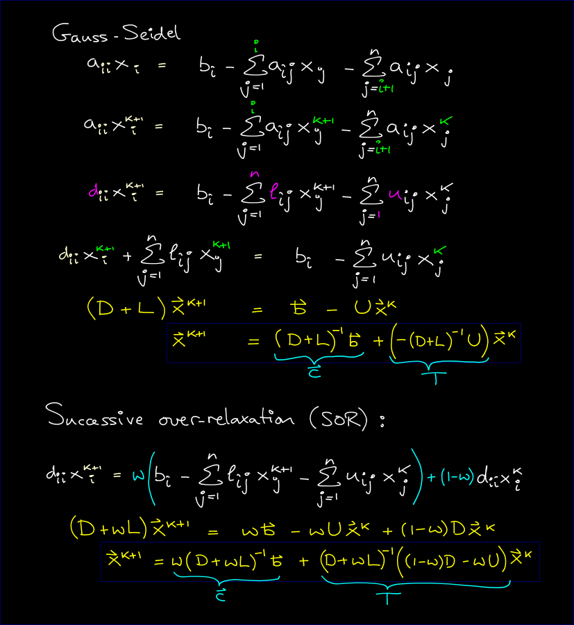
Gauss-Seidel method
Same as Jacobi except uses updated values, where available, instead of old ones. Typo alert: the green "i" in the first 2 lines should be "i-1".
#w[1:-1,1:-1] = 0.25*(w[0:-2,1:-1]+ w[2:,1:-1] + w[1:-1,0:-2]+ w[1:-1,2:]) # Jacobi - numpy makes temp array
for i in range(1,M):
        for j in range(1,N):
                w[i,j]        = 0.25*(w[i-1,j] + w[i+1,j] + w[i,j-1] + w[i,j+1] )   # Gauss-Seidel
Note the following images are have full resolution: if you want to see them in full detail, right-click View Image.
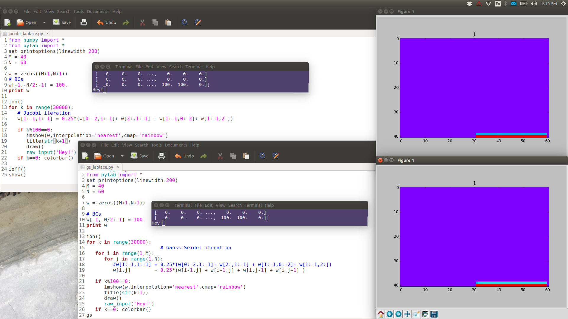
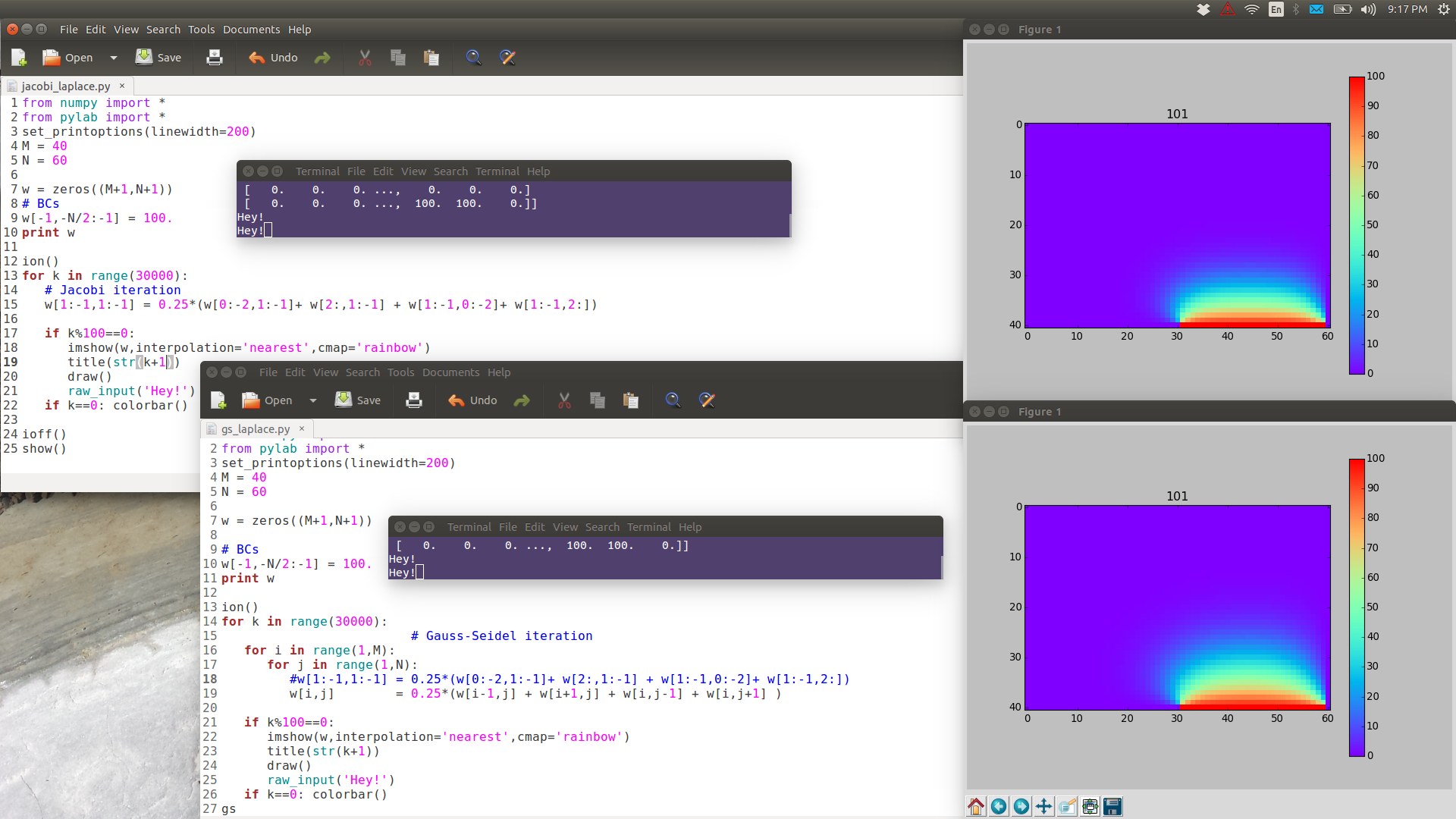
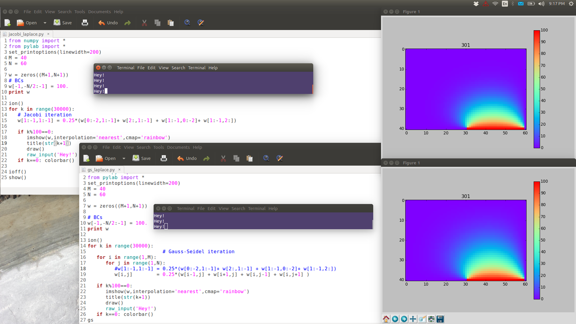
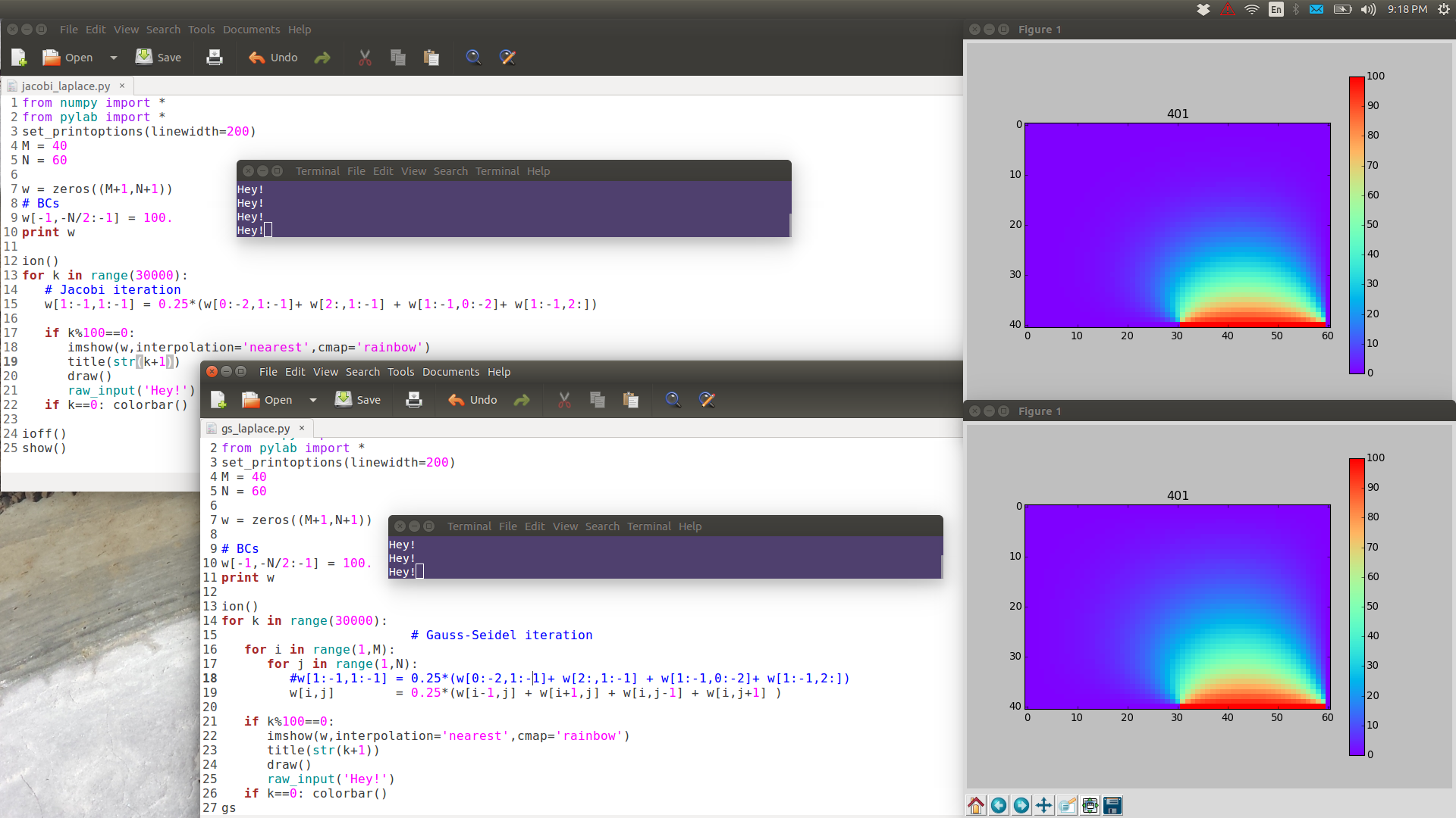
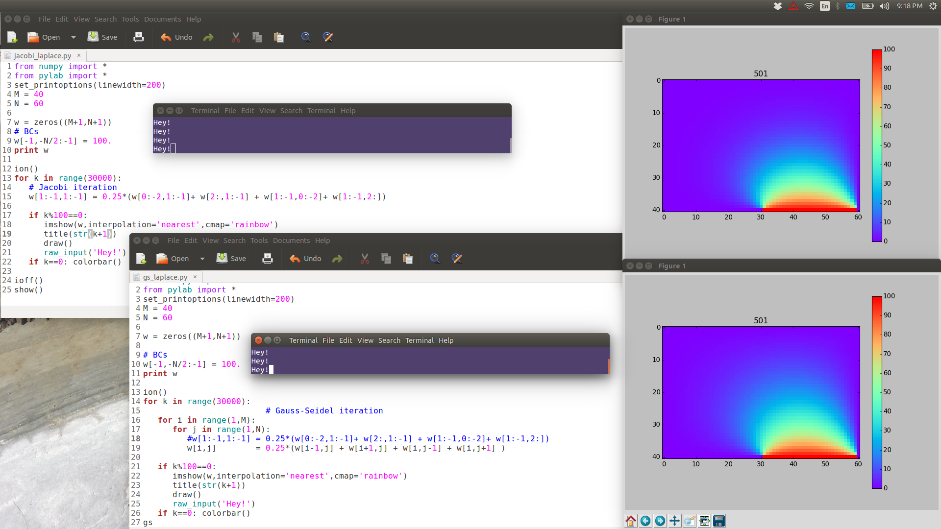
GS is noticeably faster than Jacobi.
Successive Over-Relaxation
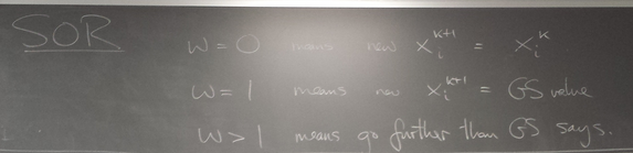
Like Jacobi, GS seems to be converging monotonically. Why not change by a bit more on each step than GS is telling us to? This idea is called SOR. We consider a linear homotopy passing through not moving at all (w=0) and the GS step (w=1).
Optimal ω: SOR (Java) demo
I wrote this Java demo some years back. It uses Java features that are now deprecated/not working. So no click responses. Need to recompile (javac) to change w value.
TODO when have time: re-implement in HTML5/Javascript:
Eigenvalues of the iteration and optimal ω
Let us explore the eigenvalues as a function of relaxation parameter ω: sor_eigenvalues.py.
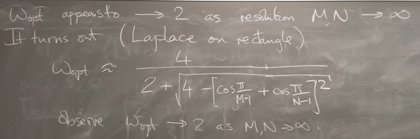
For Laplace's equation on a rectangle with M-1 by N-1 grid of interior nodes, we get as follows:

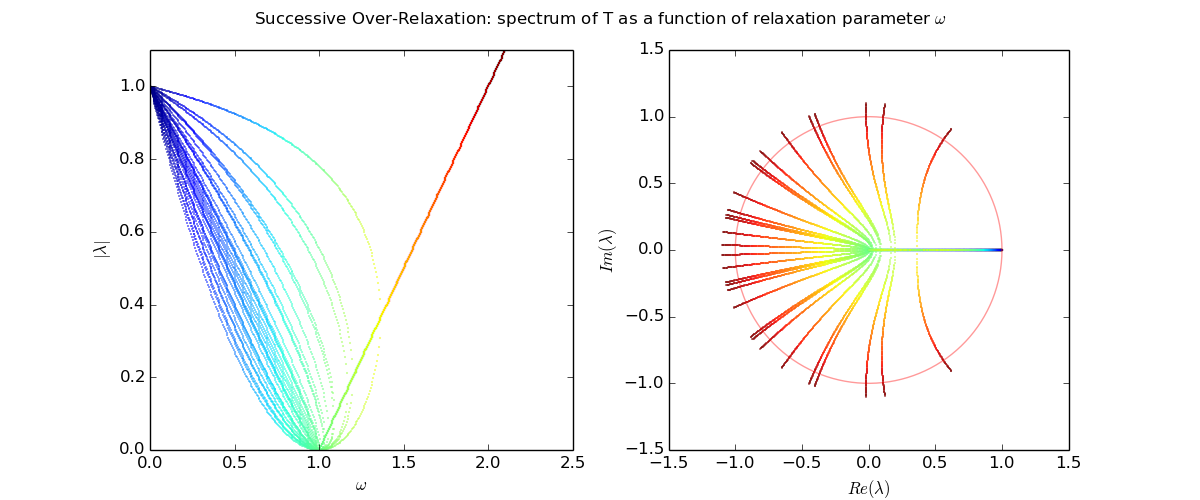
We see that as the resolution (M,N) increases, the optimal w increases towards 2, and unfortunately the spectral radius even at the optimal w approaches 1.
March 24, 2016
Discrete Fourier Transform, cont'd
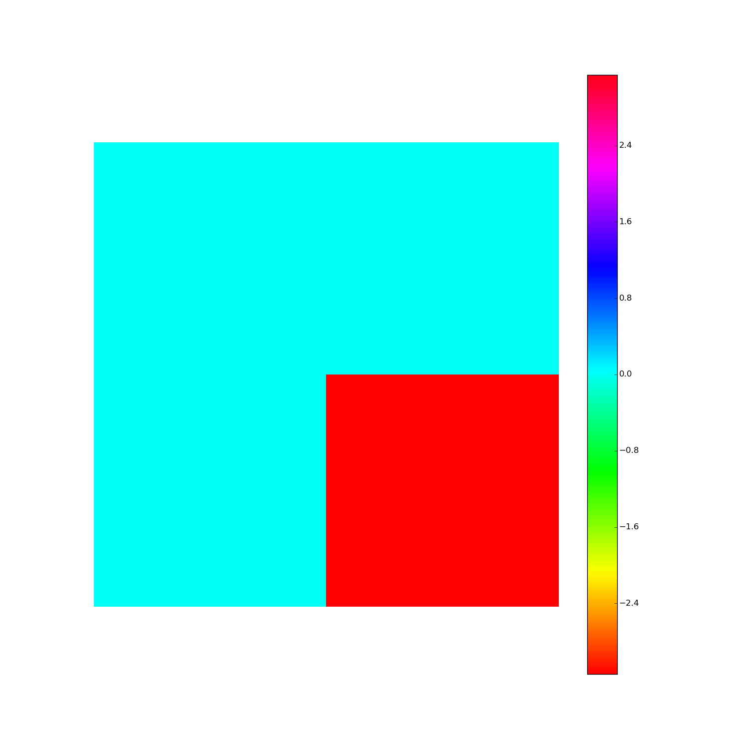
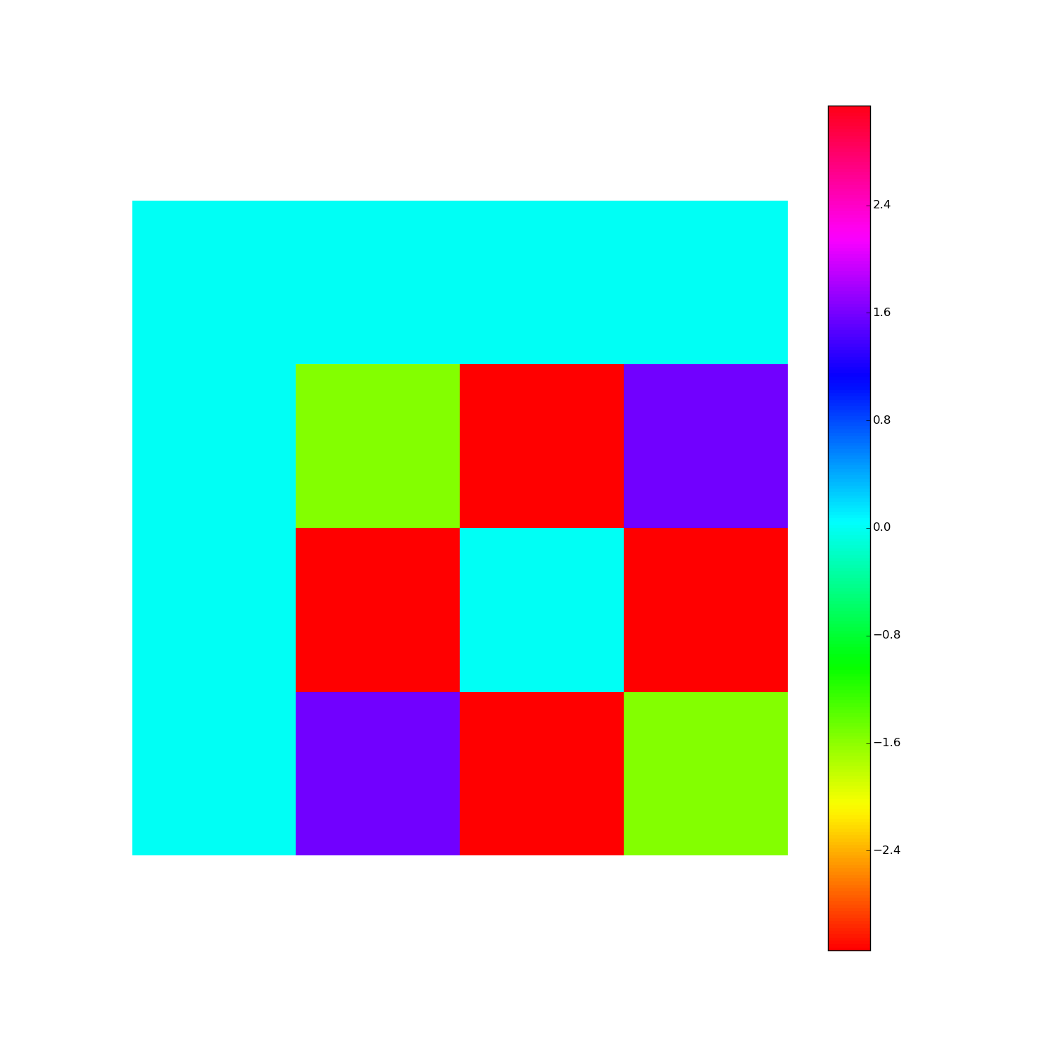
How to visualize the DFT?
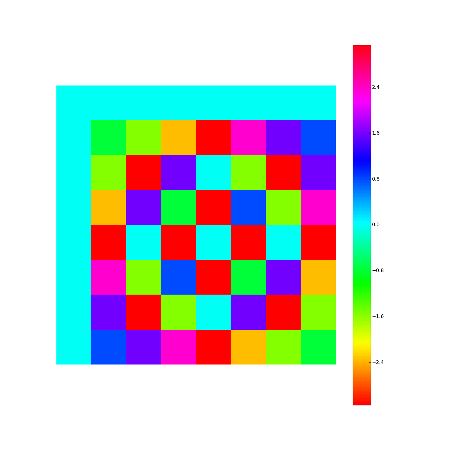
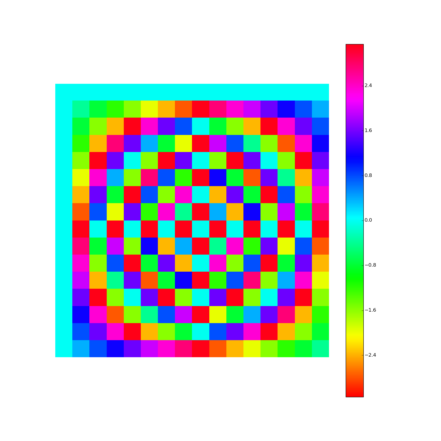
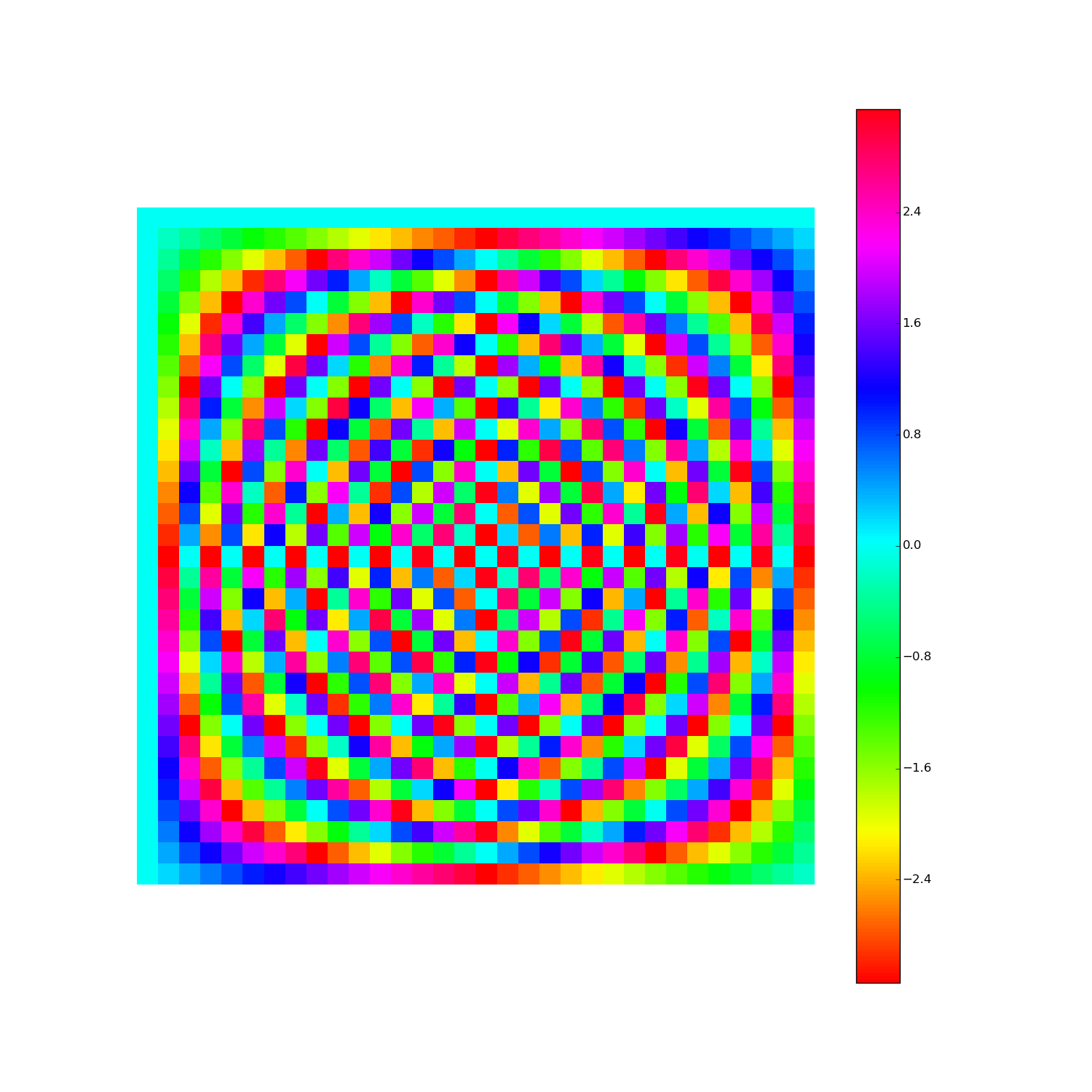
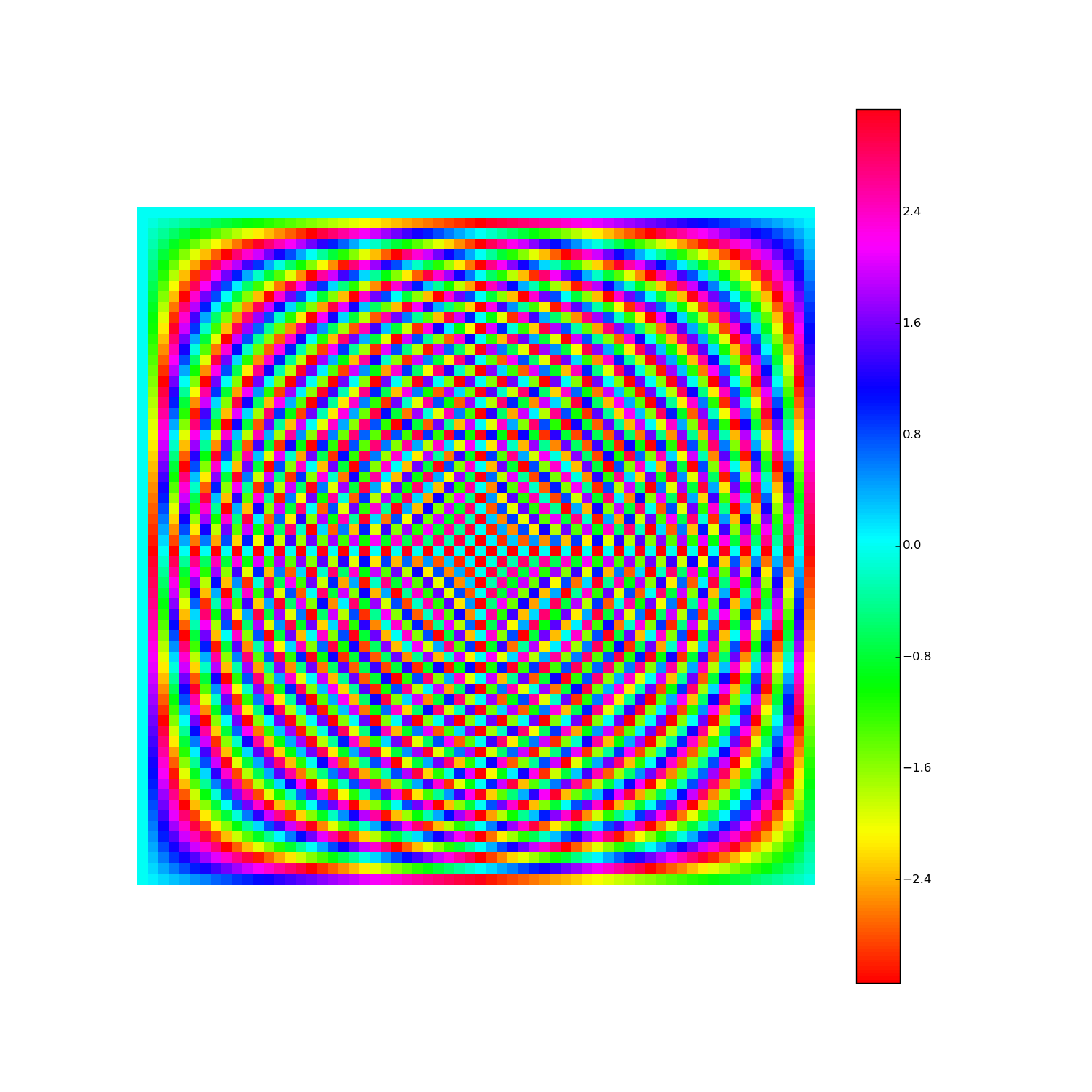
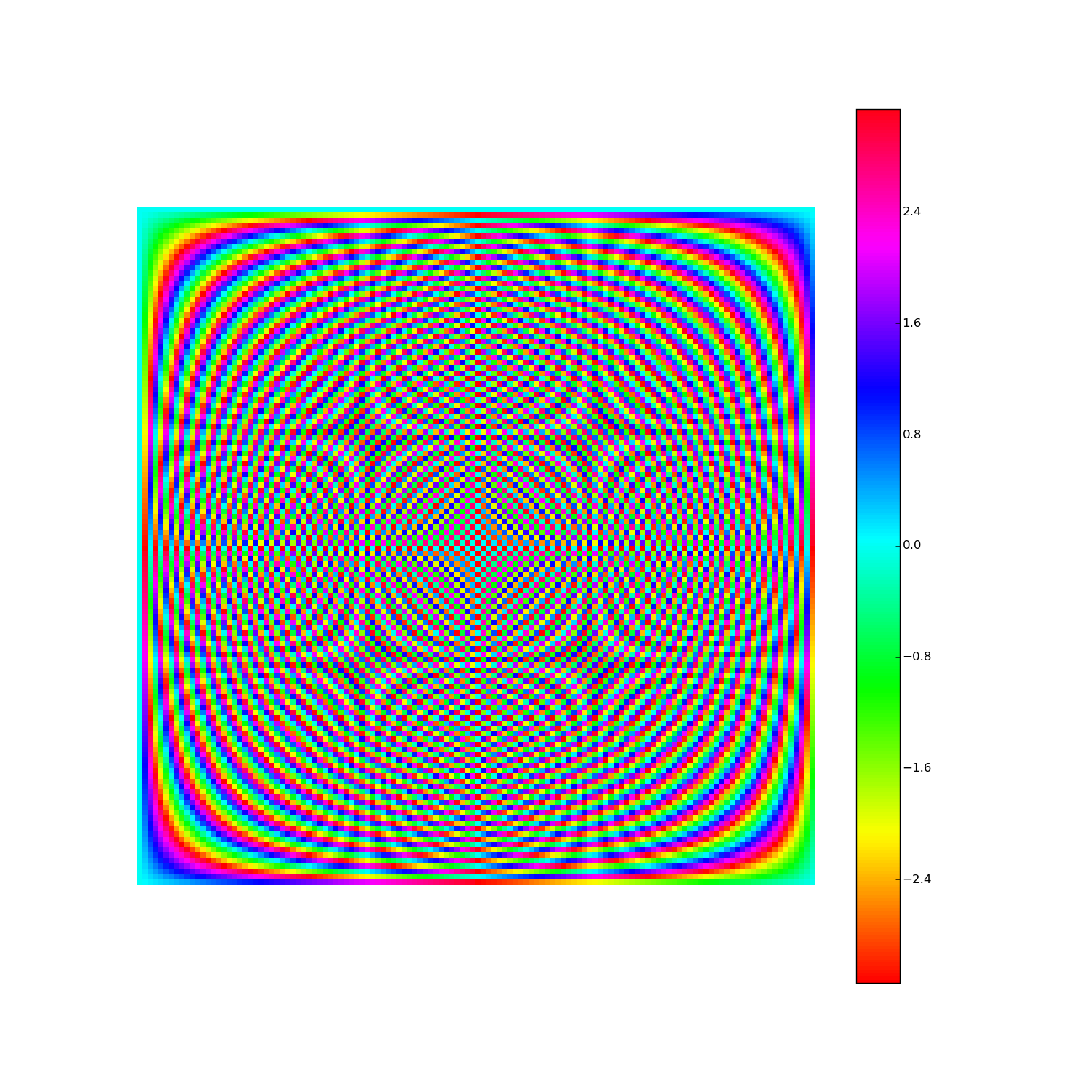
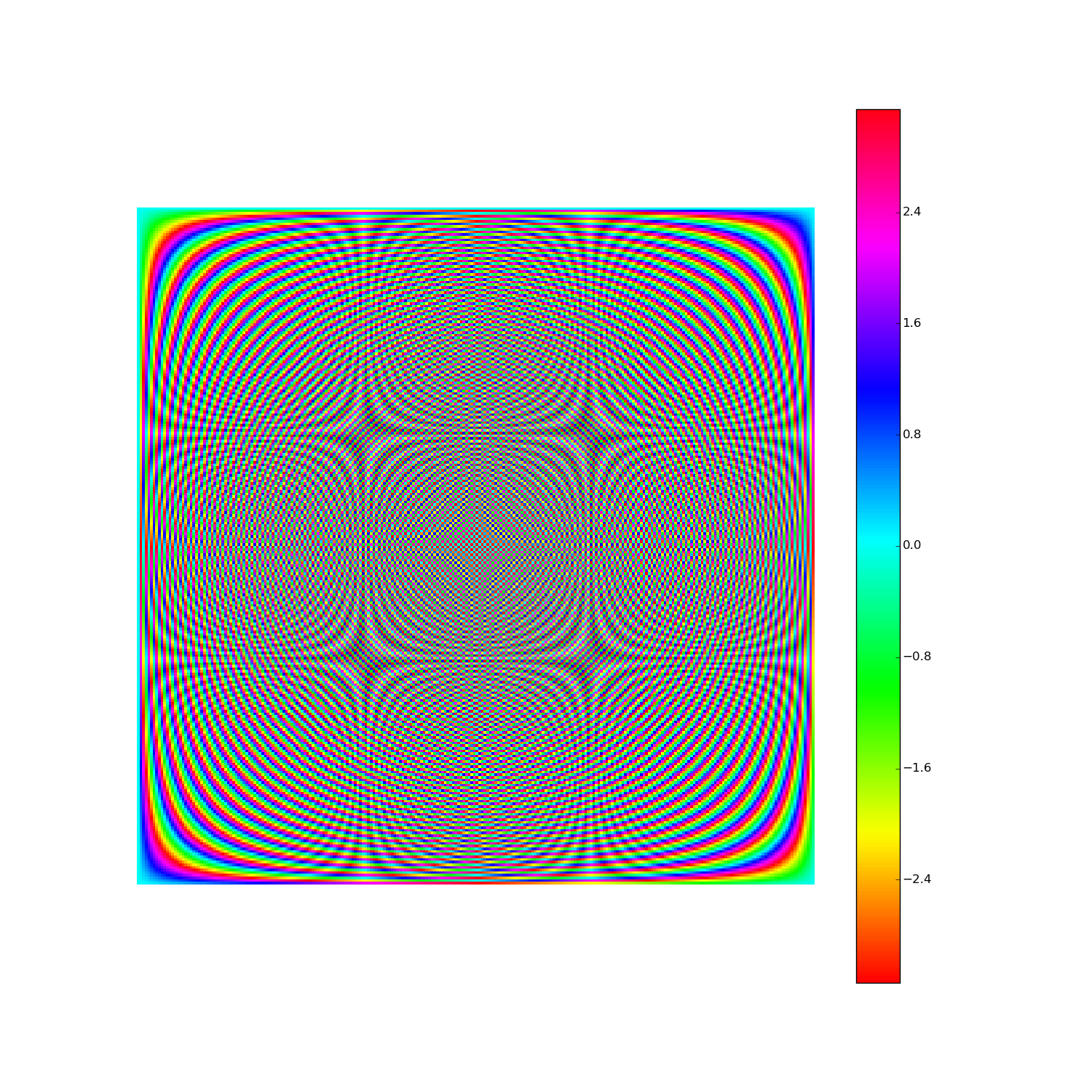
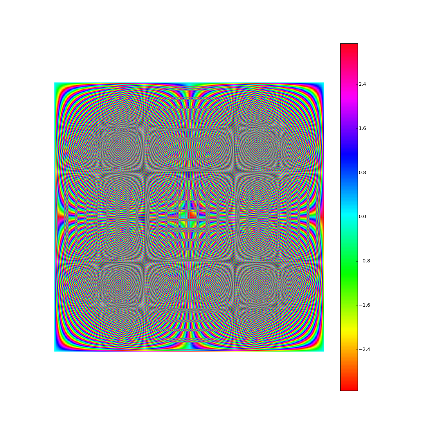
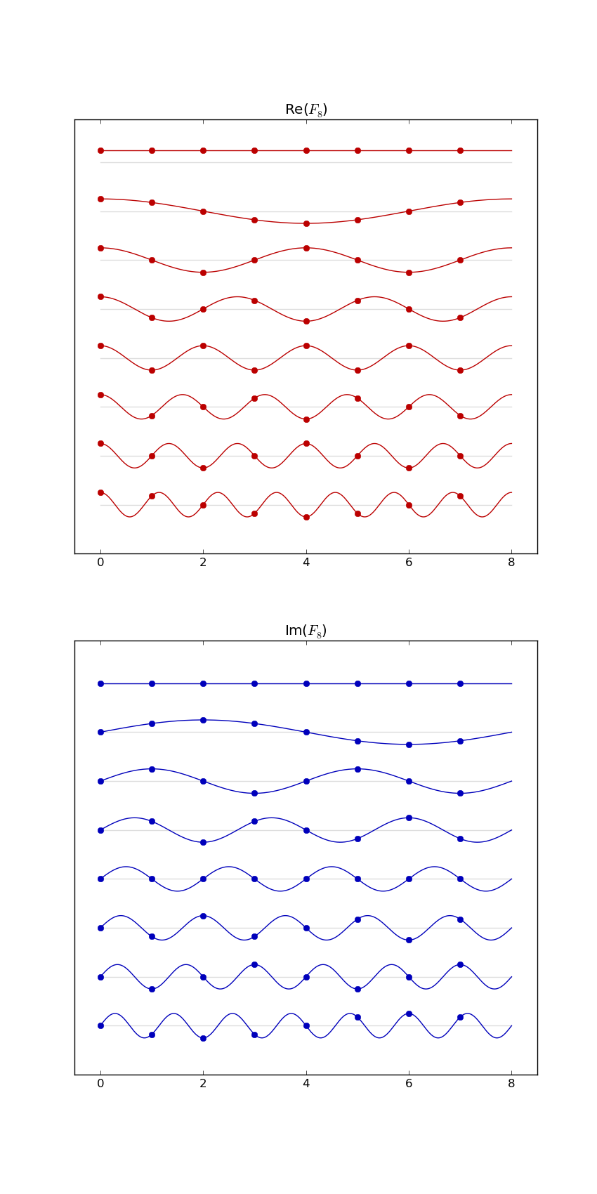
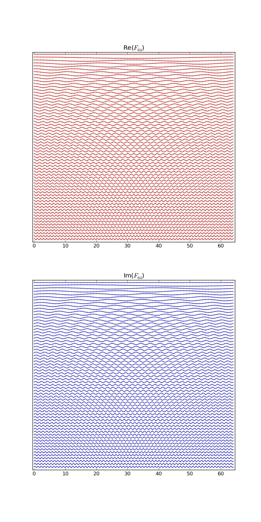
Here's F2i for i in range(1,10). Elements are eiθ with color coding θ: (Right click > View Image to see full-res version.)
Another way:
An application of DFT (piano)
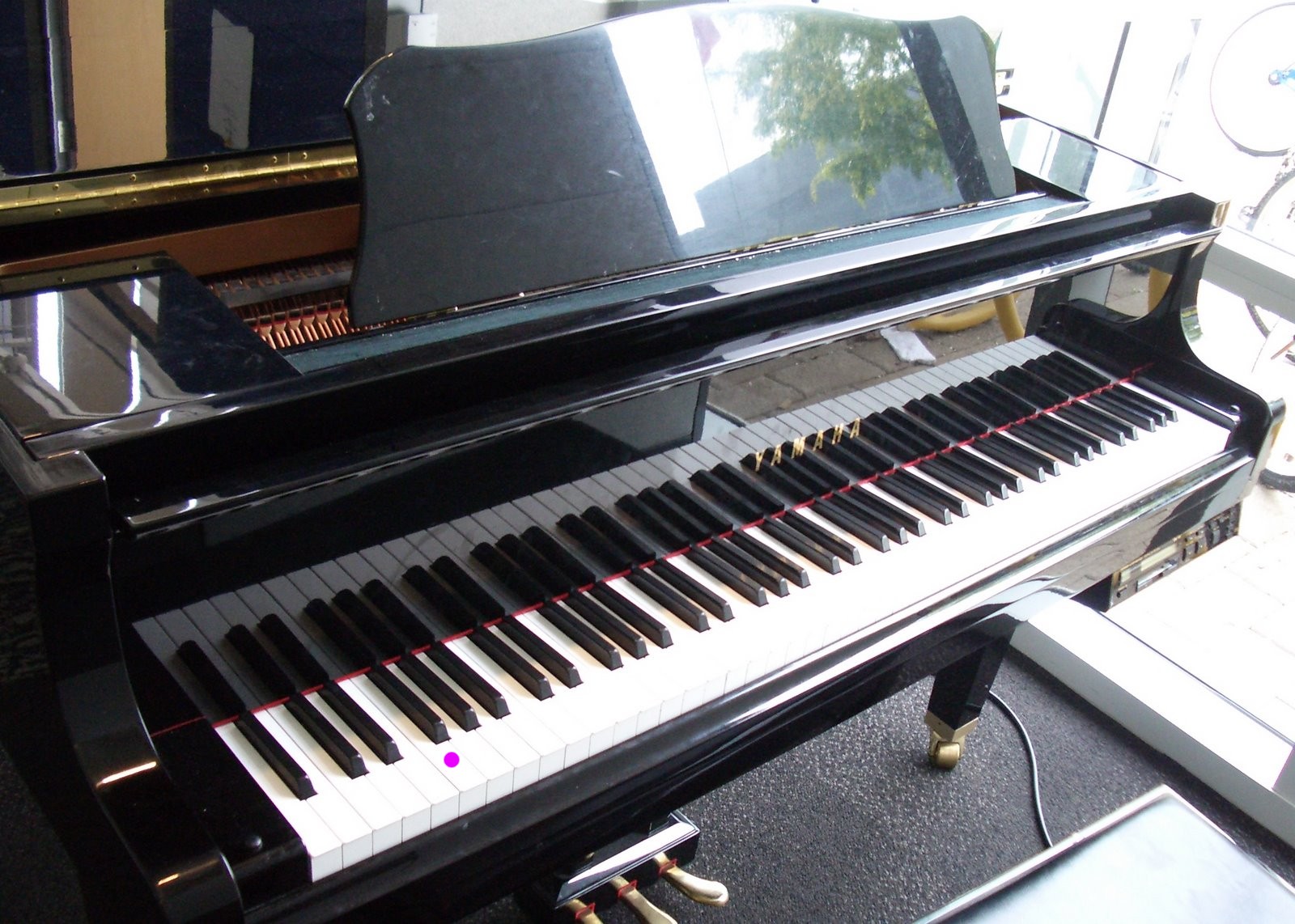
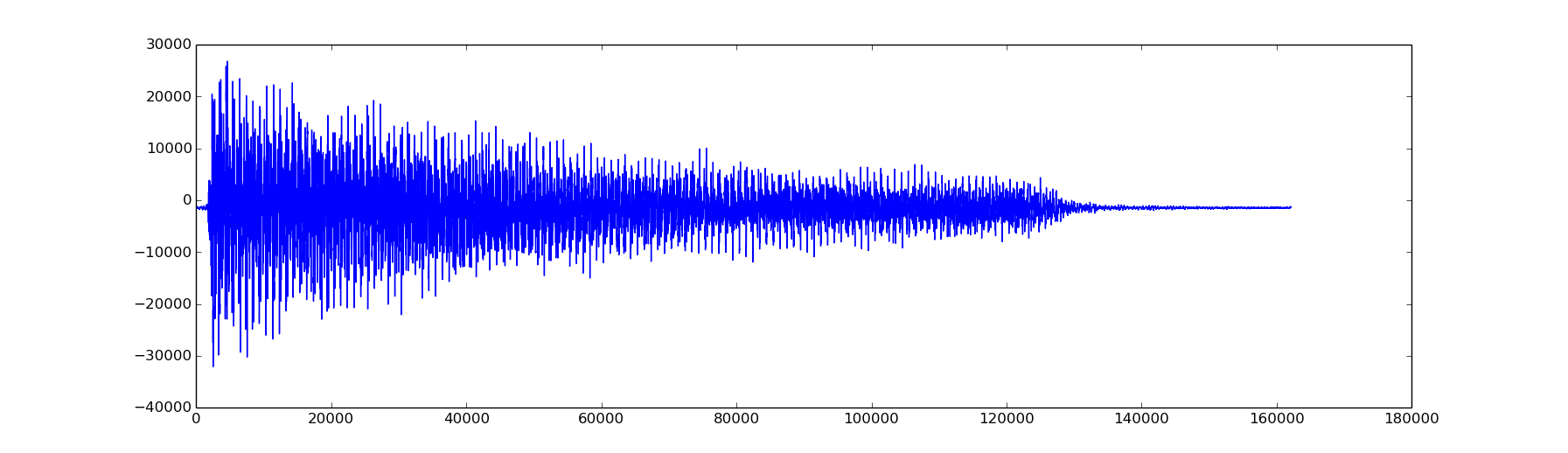
Here is a plot of the signal:
from scipy.io import wavfile
from numpy import *

rate,x = wavfile.read('piano_low_f.wav')
print 'rate',rate
print 'x.shape',x.shape

n = x.shape[0]
d = n/float(rate)  # duration of recording
print 'duration',d,'secs'

import matplotlib.pyplot as plt
plt.plot(x)
plt.show()
Next we will compute the DFT of the signal, and plot the modulus (abs) of the components of the DFT versus the corresponding frequencies.
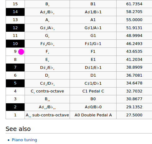
If the piano is tuned to standard "concert pitch", here are the frequencies of the notes:
Converting DFT index k to frequency
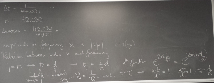
from scipy.io import wavfile
from numpy import *

rate,x = wavfile.read('piano_low_f.wav')
print 'rate',rate
print 'x.shape',x.shape

n = x.shape[0]
d = n/float(rate)  # duration of recording
print 'duration',d,'secs'

import matplotlib.pyplot as plt
#plt.plot(x)
#plt.show()

from scipy.fftpack import fft

y = fft(x)
#print type(x)

print y

# mark the nominal frequency and its harmonics (integer multiples)
f = 43.6535
for i in range(20):
        #plt.plot([i*f,i*f],[0,1.e9],'r')
        plt.axvline(i*f,color='r')

plt.plot( arange(n)/d , abs(y),'o-' )

plt.xlim(0,3000/d)
plt.xlabel('frequecy (Hz)')
plt.show()
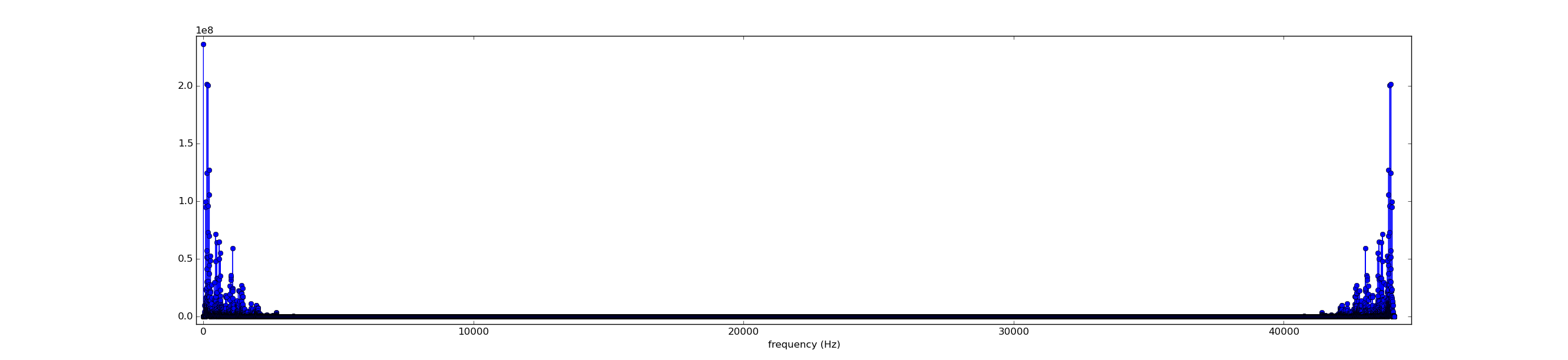
When x is a real vector, yn − k = yk for k = 1, 2, 3, ..., n − 1. Hence the moduli of yn − k and yk are equal for k = 1, 2, 3, ..., n − 1, resulting in the mirror symmetry of the above plot. Focusing on the left end, we see
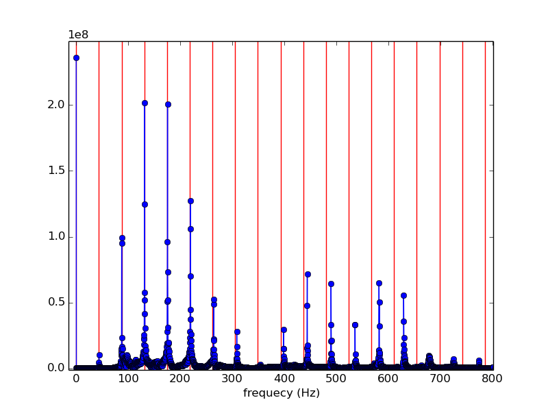
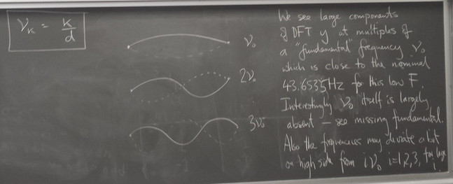
https://en.wikipedia.org/wiki/Missing_fundamental

Reiterating your observations:
March 31, 2016
Project selections
| firstname | lastname | Team # | Topic |
|---|---|---|---|
| Tiehang | Duan | 1 | Shazam |
| Anpeng | Zhang | 2 | quantum scattering |
| David | Bryant | 2 | quantum scattering |
| Neil | Heinzer | 2 | quantum scattering |
| Dante | Iozzo | 3 | heat |
| Gary | Bolduc | 3 | heat |
| Jonathan | Lottes | 3 | heat |
| Deanna | Rudik | 4 | chemical patterns |
| Eric | Davila | 4 | chemical patterns |
| Thomas | Schouten | 4 | chemical patterns |
| Jackson | Donnelly | 5 | Shazam |
| Nathan | Margaglio | 5 | Shazam |
| Sun Hyoung | Kim | 5 | Shazam |
| Le | Yang | 6 | Shazam |
| Runpu | Chen | 6 | Shazam |
| Bilal | Tariq | 7 | Shazam |
| Sean | Moran | 7 | Shazam |
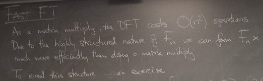
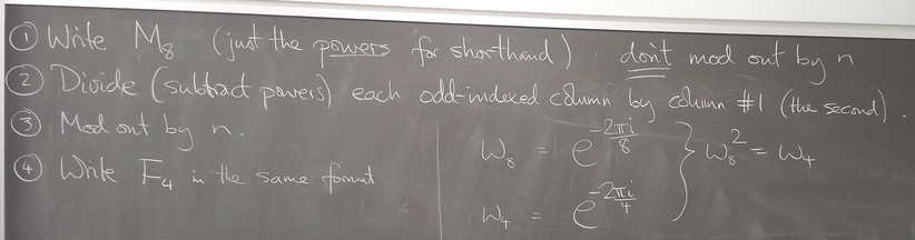
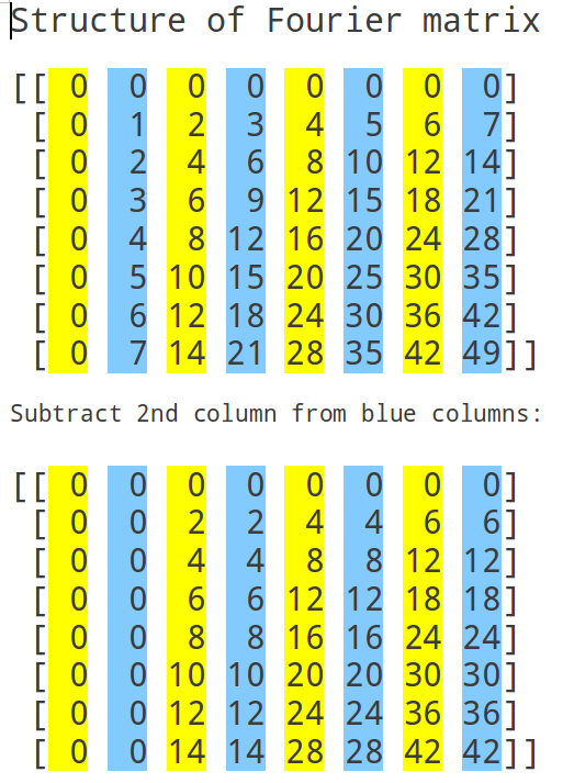
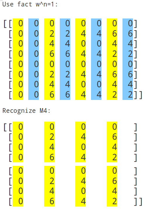
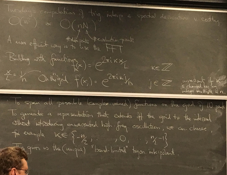
Fast Fourier Transform, cont'd
Divide and conquer
We can reexpress the DFT of x as a combination of DFTs of vectors half the size - recursively.
Implement FFT
Let's implement the FFT idea in a recursive function.
from numpy import *


def myfft(x):

        # assume that len(x) is power of 2

        n = len(x)
        if n==1: return array(x, dtype=complex)

        yeven = myfft( x[ ::2] )
        yodd  = myfft( x[1::2] )

        # now need to multiply by appropriate powers of w
        w = exp(-2j*pi/float(n))
        W = w**range(n)

        return hstack( [ yeven + W[:n/2]*yodd , yeven + W[n/2:]*yodd  ] )

        # a revolution!!!!
It's that simple!
Let's test it.
'''
x = array([2.,4,6,8])
y = myfft(x)
print y
'''
j = 16
x = random.rand(2**j)-0.5
y = myfft(x)             # my fft

# compare with scipy's fft

from scipy.fftpack import fft
npy = fft(x)             # scipy's fft
# are they the same?
print 2**j, sum(abs(y-npy)/linalg.norm(npy)), 'should be very close to zero'
$ python myfft.py
1024 4.33461856145e-13 should be very close to zero
Agrees closely with scipy's fft.
Operation count for FFT
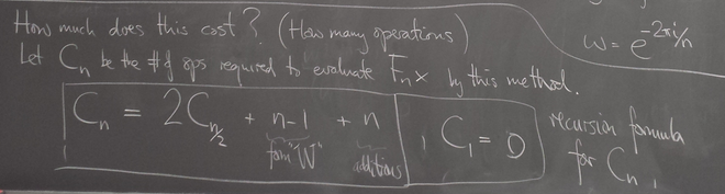
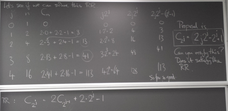
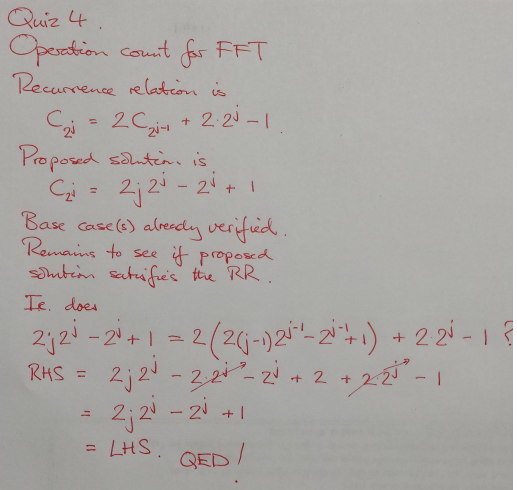
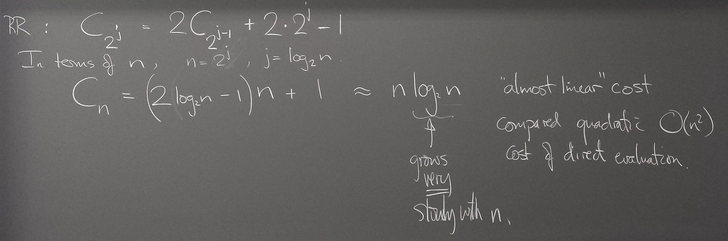
We find the cost of FFT is ~ n log n instead of ~ n^2 for direct matrix multiplication
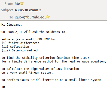
Exam 2
Exam 2 is this Thursday, April 7. It covers everything from where we left off in Exam 1 through the Fast Fourier Transform.
That includes finite-difference, collocation, and Galerkin methods for ODE BVPs; finite difference methods for parabolic, elliptic and hyperbolic 2nd order PDEs; Jacobi, Gauss-Seidel and SOR iteration for solving linear systems; the DFT and FFT.
You may bring a non-programmable non-graphing scientific calculator, and handwritten notes on a single copy of the personalized note sheet I emailed you a link to on April 4.
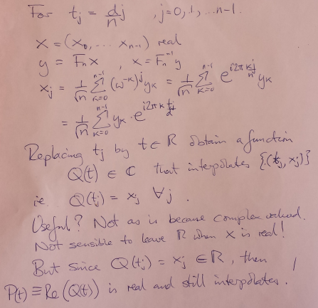
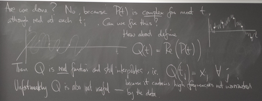
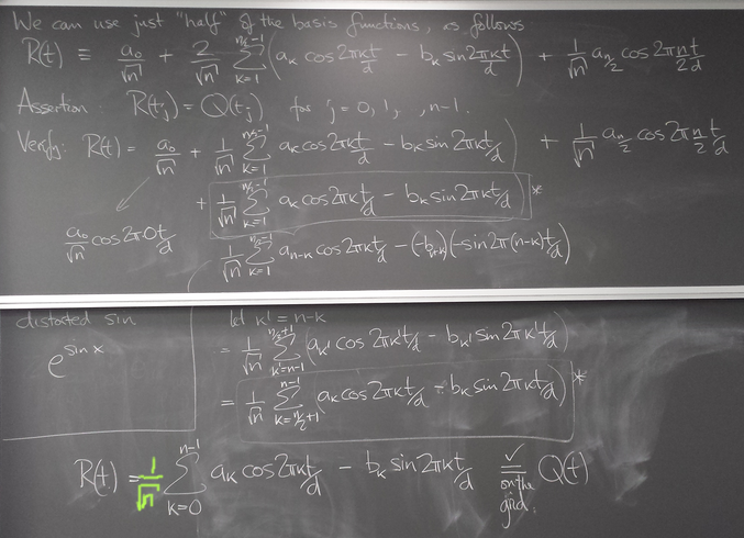
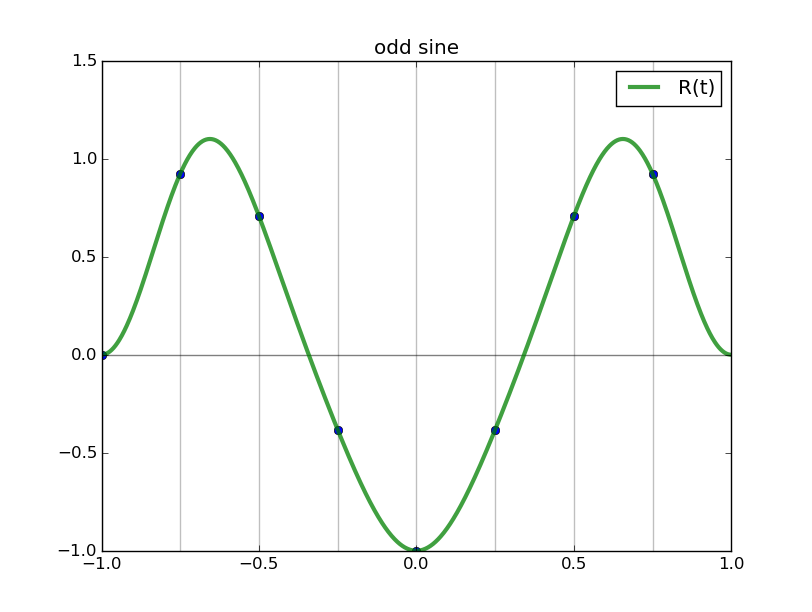
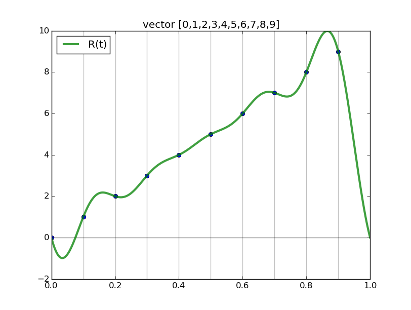
Trigonometric interpolation, cont'd
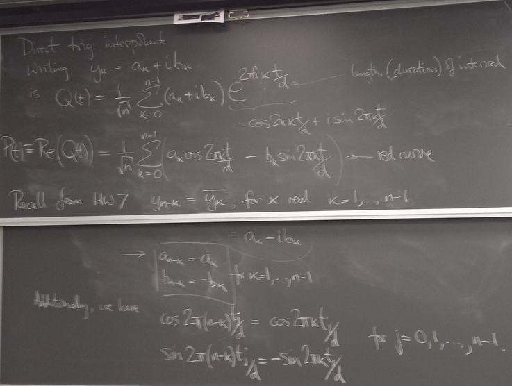
Real part of raw "continuized" IDFT unsuitable (high-frequencies)
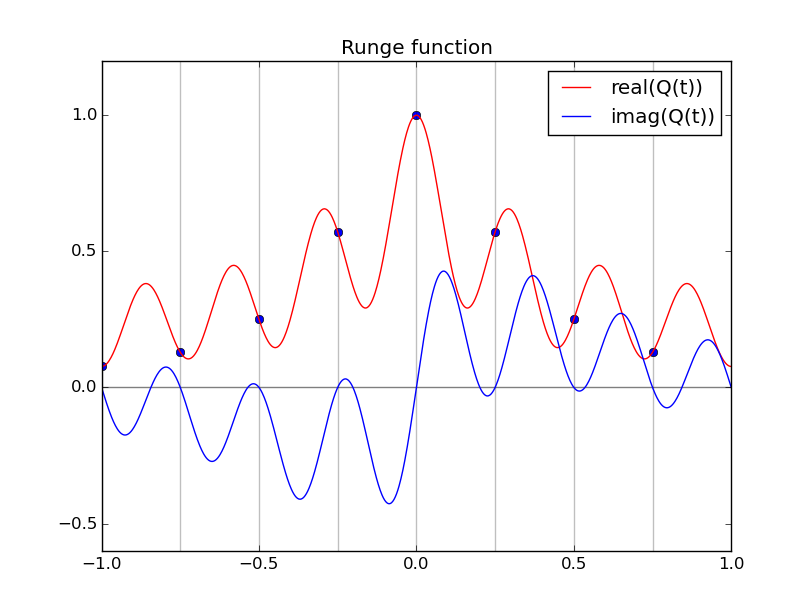
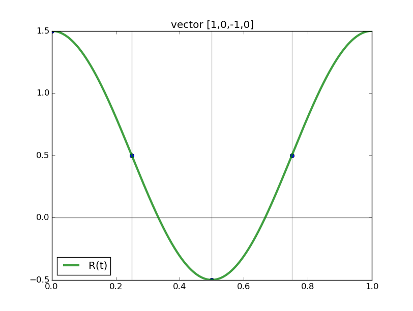
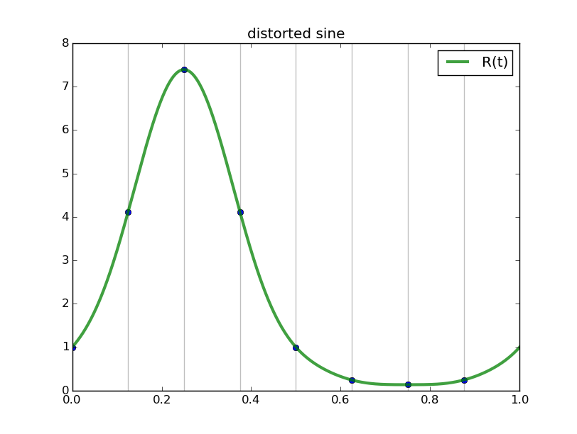
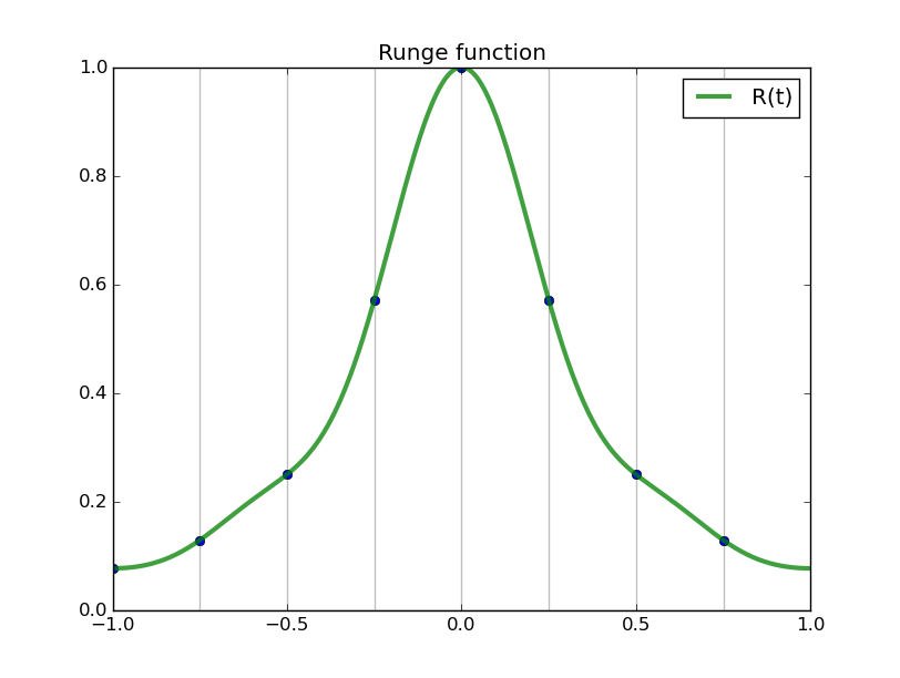
#triginterp.py
from numpy import *
from scipy.fftpack import fft,ifft
from pylab import plot,ion,ioff,draw,title,figure,axvline,legend

formula = 'Q'

for example in [3]:#range(1,4):

        figure(example)
        if example==1:
                mytitle = 'vector [1,0,-1,0]'
                c = 0.
                d = 1.
                L = d-c
                x = array([1.,0.,-1.,0.])+0.5
                n = len(x)
                t = L*arange(n)/float(n)
        elif example==2:
                mytitle = 'distorted sine'
                n = 8
                c = 0.
                d = 1.
                L = d-c
                t = linspace(0.,L,n,endpoint=False)
                print len(t)
                def myf(t): return exp(2.*sin(2*pi*t/L))#sin(2*pi*t/L)#
                x = myf(t)
        elif example==3:
                mytitle = 'Runge function'
                n = 8
                c = -1.
                d =  1.
                L = d-c
                t = linspace(c,d,n,endpoint=False)
                print len(t)
                def myf(t): return 1/(1+12.*t*t)
                x = myf(t)

        elif example==4:
                mytitle = 'odd sine'
                n = 8
                c = -1.
                d =  1.
                L = d-c
                t = linspace(c,d,n,endpoint=False)
                print len(t)
                def myf(t): return sin(3*pi*(t-c)/L)
                x = myf(t)

        elif example==5:
                mytitle = 'vector [0,1,2,3,4,5,6,7,8,9]'
                c = 0.
                d = 1.
                L = d-c
                x = array([0,1,2,3,4,5,6,7,8,9],dtype=float)
                n = len(x)
                t = L*arange(n)/float(n)

        else:
                print "Which example do you want me to do?"

        ion()
        plot( t, x, 'o')
        for tj in t: axvline(tj,color='k',alpha=0.25)

        y = fft(x)/sqrt(n) # division to get Sauer def of DFT
        a = real(y)
        b = imag(y)
        print 'y',y
        print 'a',a
        print 'b',b

        tt = linspace(c,d,1000)
        #plot(tt,myf(tt),'k')
        plot([c,d],[0,0],'k',alpha=0.5)

        p = zeros_like(tt,dtype=complex)
        for k in range(n):
                p += y[k]/sqrt(n)*exp(complex(0.,1.)*2.*pi*k*(tt-c)/L)
        plot(tt,real(p),'r',label='real(Q(t))')
        plot(tt,imag(p),'b',label='imag(Q(t))')

        if formula=='R':
                p = ones_like(tt)*a[0]/sqrt(n)
                for k in range(1,n/2):
                        p += 2./sqrt(n)*( a[k]*cos(2*pi*k*(tt-c)/L) - b[k]*sin(2*pi*k*(tt-c)/L) )
                p += a[n/2]/sqrt(n)*cos(n*pi*(tt-c)/L)
                plot(tt,p,'g',linewidth=3,alpha=0.75)
        elif formula=='P':
                p = zeros_like(tt)
                for k in range(0,n):
                        p += 1./sqrt(n)*( a[k]*cos(2*pi*k*(tt-c)/L) - b[k]*sin(2*pi*k*(tt-c)/L) )
                plot(tt,p,'g',linewidth=3,alpha=0.75)

        legend()
        title(mytitle)
        draw();

ioff(); raw_input("")
Symmetries for real x
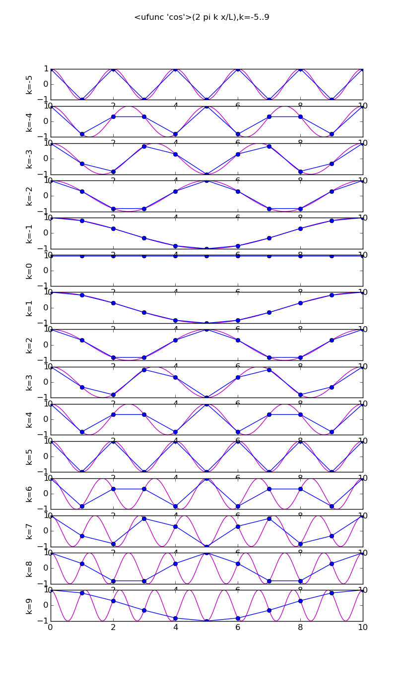
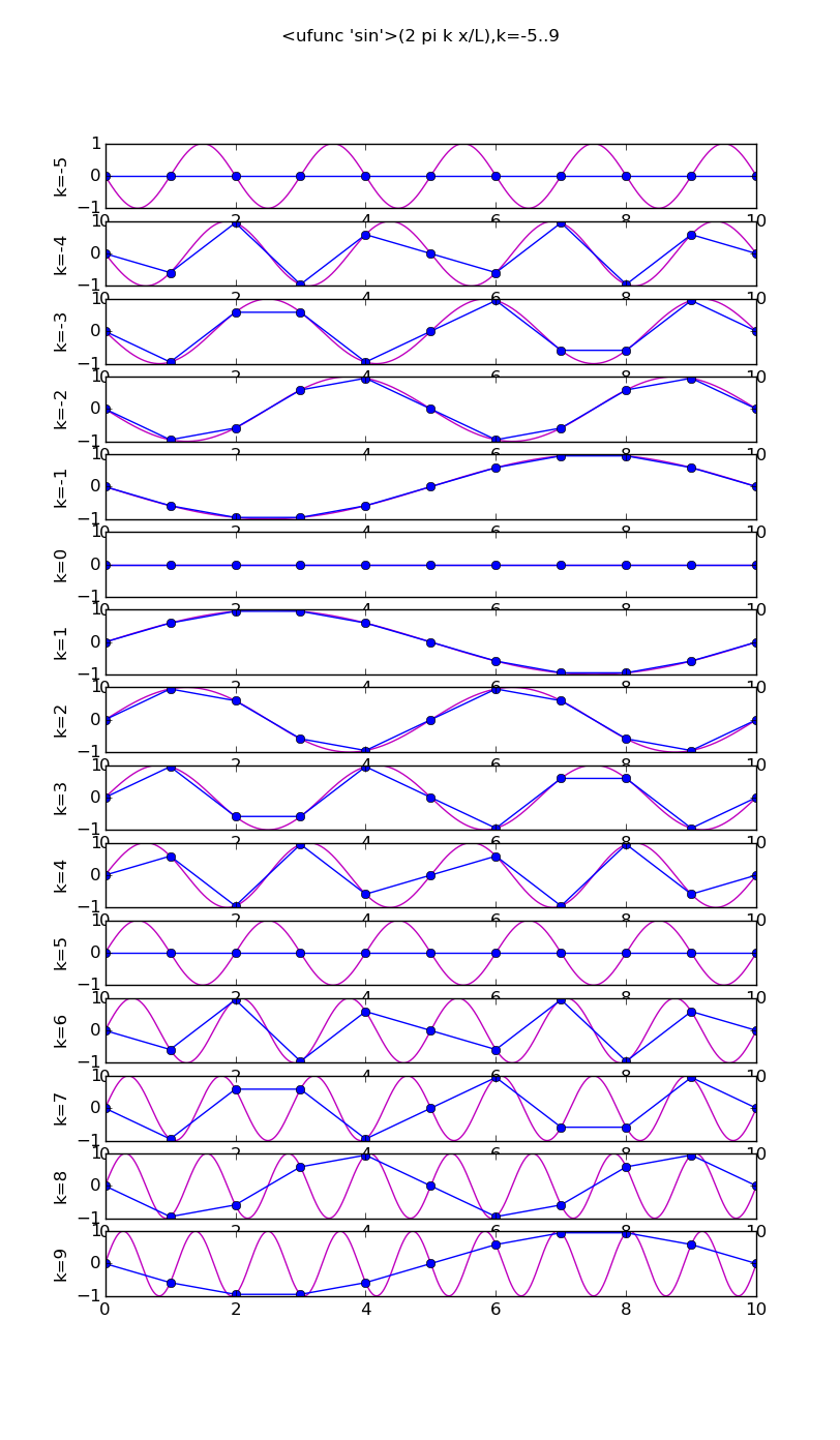
There exist symmetries in the coefficients and the basis functions restricted to the grid, that enable us to obtain an interpolant involving only the lower half of the frequency components.
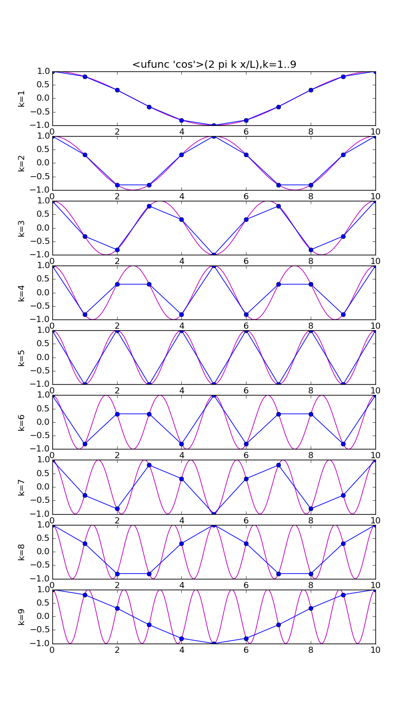
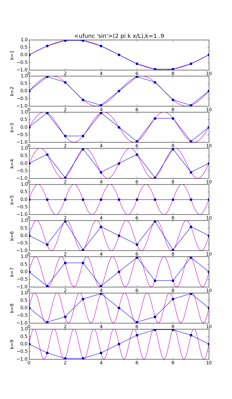
# modes.py
from pylab import *
from numpy import *
n = 10
j = array(range(n+1))
x = linspace(0,n,1000)
ion();

for f in [cos,sin]:
        figure(str(f),figsize=(8,16))
        for k in range(1,n):
                subplot(n-1,1,k)
                vv = f(2*pi*k*x/float(n))
                v  = f(2*pi*k*j/float(n))
                plot(x,vv,'m')
                plot(j, v,'bo-')
                ylabel('k='+str(k))
                if k==1: title(str(f)+'(2 pi k x/L),k=1..'+str(n-1))

draw(); ioff(); raw_input()
Interpolation examples
Observe the nice interpolants R(t) we get (using the code above but with formula='R', and the red and blue curves omitted):
Spectral differentiation
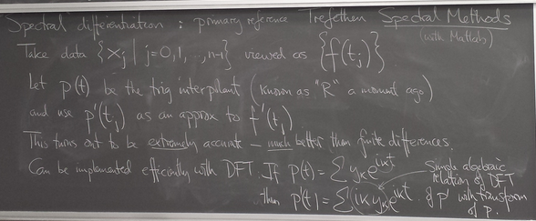
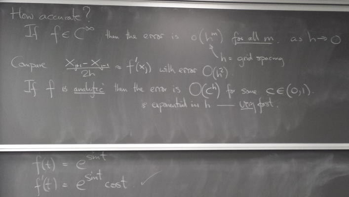
Trefethen code (translated to python) to compute the spectral derivative (using FFT): p5.py.
Here we see the function f(t) = exp(sin(t)), the trigonometric interpolant to its sampling on grids of various refinement, and the corresponding spectral derivative compared with the true derivative:
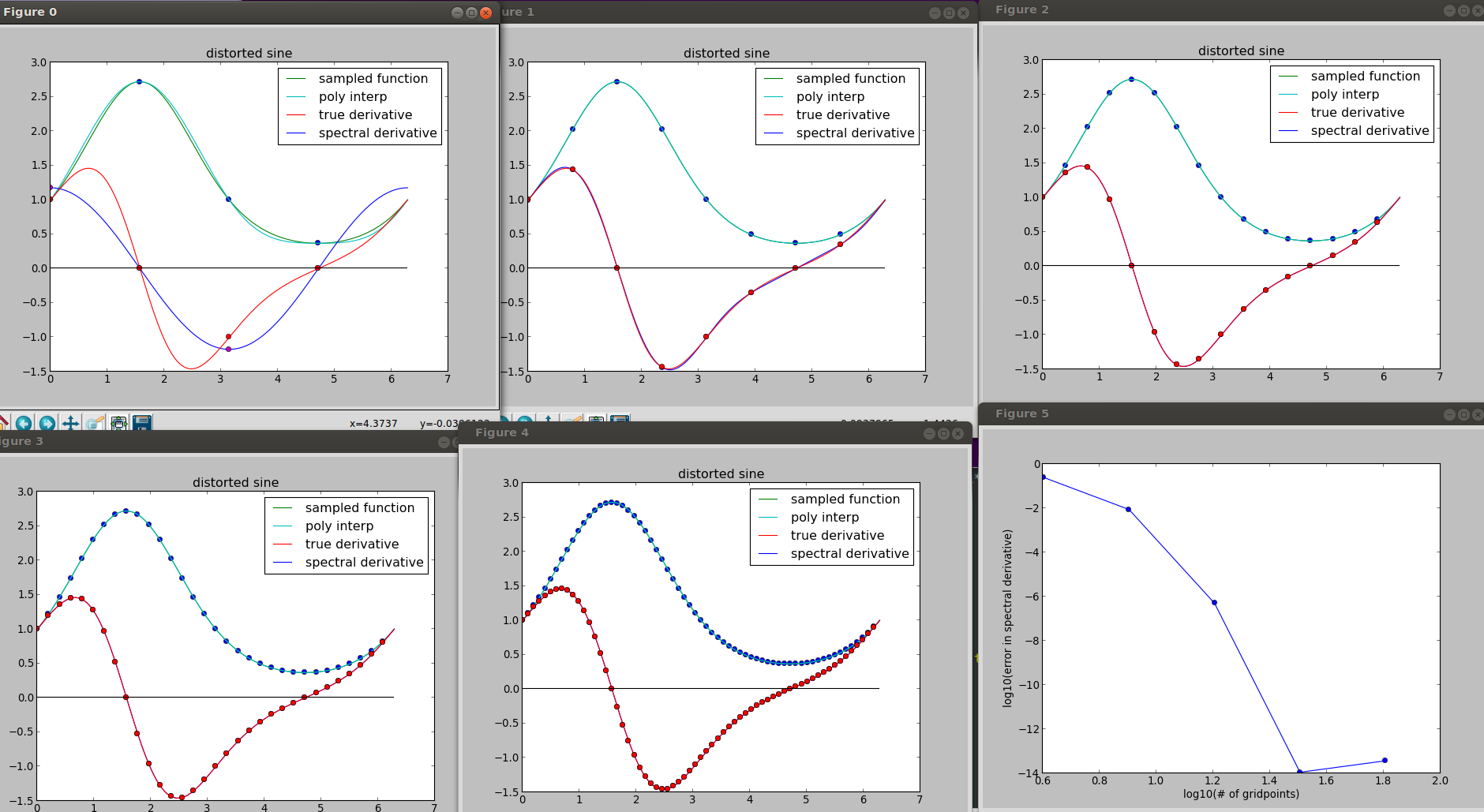
The error is log-log-plotted in the last frame. See how fast it decreases as the grid is refined. Compare with finite_diff_derivative.py: we have (shallow) straight lines on the corresponding plot.
Spectral derivatives, cont'd
Accuracy of spectral derivative
Your turn! Starting with the code below, also linked here, fill in all the blanks to assess the quality of spectral differentiation.
#spectraldiff.py

from numpy import *
from scipy.fftpack import fft,ifft
import matplotlib.pyplot as plt

mytitle = 'distorted sine'
c = 0.
d = 3.
def myf(t): return exp(2.*sin(2*pi*t/L))
#def myfprime(t): return # supply exact derivative here

L = d-c

for n in [8,16]:

        plt.figure(n)
        t = linspace(0.,L,n,endpoint=False)

        x = myf(t)

        # plot the data x
        for tj in t: plt.axvline(tj,color='k',alpha=0.25)
        plt.plot( t, x, 'o')

        # get DFT of x
        y = fft(x)
        a = real(y)
        b = imag(y)

        # form trigonometric interpolant (refer to notes: http://blue.math.buffalo.edu/438/trig_interp_apr5_chalk_2.png)

        tt = linspace(c,d,1000)  # dense grid
        p = zeros(n)

        # plot trigonometric interpolant along with actual function


        # print norm of error in the trigonometric interpolant


        # compute and plot the interpolation error


        # form derivative of trigonometric interpolant


        # plot derivative of trigonometric interpolant and of actual function


        # compute and plot the error in the spectral derivative

        # print norm of error in the spectral derivative
        plt.title(mytitle + ': '+str(n)+' sample points')

plt.show()
Upload your code to UBlearns.
That's as far as we got on April 12, 2016.
April 14, 2016
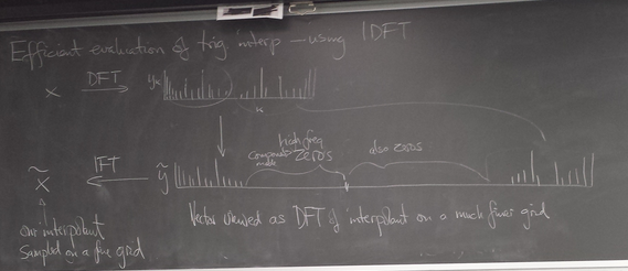
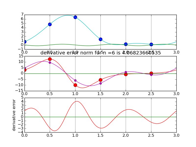
More efficient evaluation of trig interpolant and spectral derivative using IFFT
Another view using negative wave numbers. Illustration for n=10.
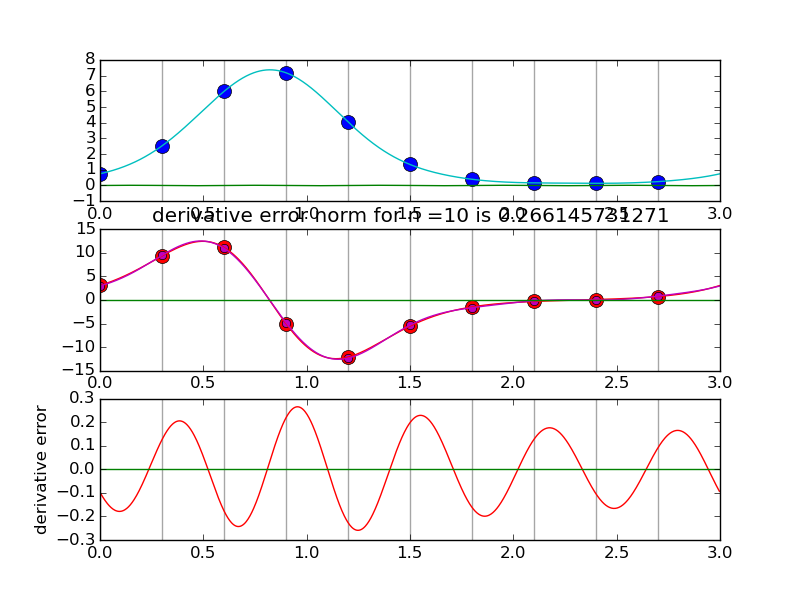
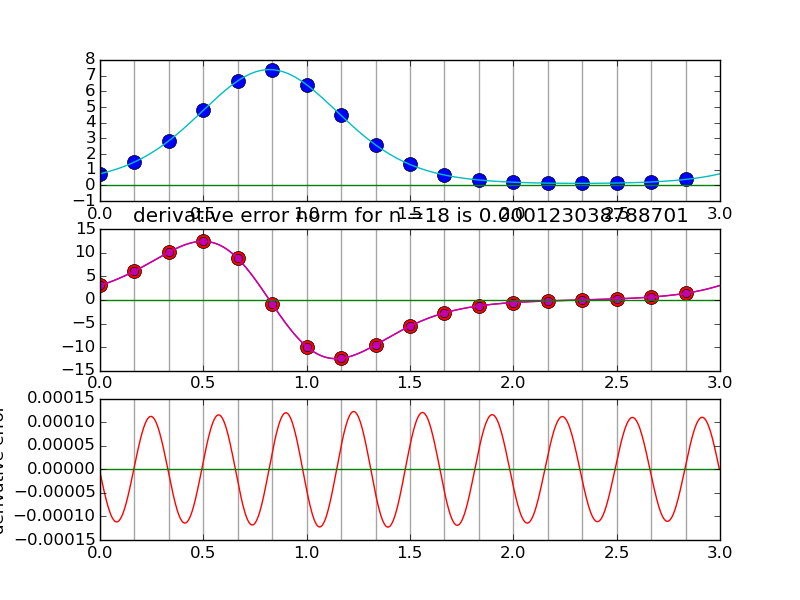
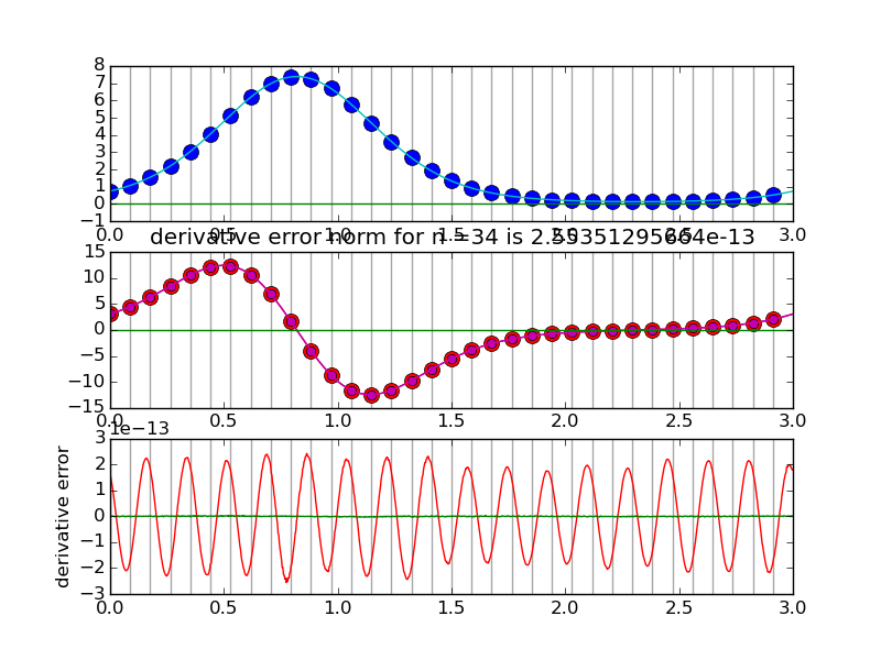
#spectraldiff_fft.py

from numpy import *
from scipy.fftpack import fft,ifft
import matplotlib.pyplot as plt
import sys

mytitle = 'distorted sine'
c = 0.
d = 3.
shift = 0.07
def myf(t): return exp(2.*sin(2*pi*(t-shift)/L))
def myfprime(t): return exp(2.*sin(2*pi*(t-shift)/L))*2.*cos(2*pi*(t-shift)/L)*(2*pi/L)

L = d-c

nvals = [2+2**i for i in range(2,6)]

N = 1000  # grid for evaluating interpolant
T = linspace(0.,L,N,endpoint=False)

for i,n in enumerate(nvals):
        plt.clf()
        t = linspace(0.,L,n,endpoint=False)

        x = myf(t)  # get the data

        plt.subplot(3,1,1)
        # plot the data x
        for tj in t: plt.axvline(tj,color='k',alpha=0.35)
        plt.plot( t, x, 'bo',markersize=10)

        y = fft(x)
        Y = zeros(N,dtype=complex)
        Y[:n/2]  = y[:n/2]
        Y[-n/2:] = y[-n/2:]
        X = ifft(Y)*(N/float(n))
        #print X
        plt.plot(T,real(X),'c')
        plt.plot(T,imag(X),'g')

        k = hstack( [ range(n/2),  [0]  , range(-n/2+1,0) ] )
        #print k
        yp = y*2*pi*1.j*k/L
        print y[n/2],yp[n/2]
        xp = ifft(yp)

        plt.subplot(3,1,2)
        for tj in t: plt.axvline(tj,color='k',alpha=0.35)
        plt.plot(t,myfprime(t),'ro',markersize=10)      # true derivative of sampled f
        plt.plot(t,real(xp),'mo')

        # extend derivative to X

        YP = zeros(N,dtype=complex)
        YP[:n/2]  = yp[:n/2]
        YP[-n/2:] = yp[-n/2:]
        XP = ifft(YP)*(N/float(n))
        #print X
        plt.plot(T,myfprime(T),'r')     # true derivative of sampled f
        plt.plot(T,real(XP),'m')
        plt.plot(T,imag(XP),'g')

        plt.title('derivative error norm for n ='+str(n)+' is ' +str( linalg.norm(real(XP)-myfprime(T),inf) ) )

        plt.subplot(3,1,3)
        for tj in t: plt.axvline(tj,color='k',alpha=0.35)
        plt.plot(T,real(XP)-myfprime(T),'r')    # true derivative of sampled f
        plt.plot(T,imag(XP),'g')
        plt.ylabel('derivative error')
        plt.savefig(sys.argv[0]+'.pngs/n'+str(n).zfill(3)+'.png')
Solving advection equation using spectral spatial derivative
Using spectral derivatives can yield much better approximations to solutions of PDES than finite differences. An example is the advection equation with a space-varying advection speed.
Theory of solutions
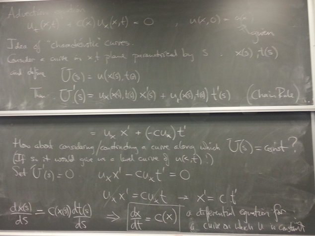
Characteristics: consider curves x(s), t(s) along which
is constant. Such curves satisfy
Implementation and test
Example:
on [0, 2π).
Leapfrog scheme
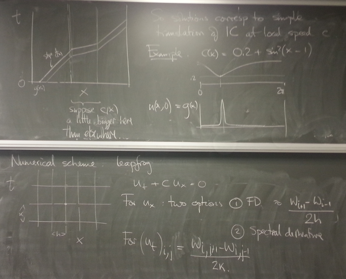
April 19, 2016
L = 2*pi, n = 128, h = L/n, k = h/4, T = 8., plot every 12th step
Utility function: waterfall.py. waterfall() wants snapshots in rows.
With finite difference spatial derivative: [let's write from scratch]
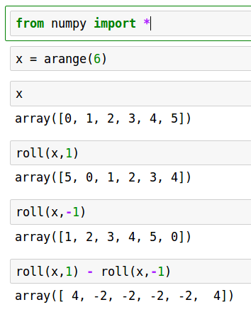
# advection_fd.py

from numpy import *
from waterfall import waterfall
import matplotlib.pyplot as plt

# spatial grid
L = 2*pi
n = 128
h = L/float(n)

# time grid
T = 8.
k = h/4.
m = int(T/k)  # number of time steps
plotskip = 12  # plot every 12th time step

w = empty((m+1,n))

def g(x): return exp( -100.*(x-1.)**2 )  # initial condition

def c(x): return 0.2 + sin(x-1)**2

x = linspace(0,L,n,endpoint=False)
cgrid = c(x)

w[0,:] = g(x)
# quick and dirty first step
w[1,:] = g(x-k*c(1.))  # just shift by speed at x=1

for j in range(1,m):
        # spatial derivative approximation at row j
        wx =  ( roll(w[j,:],-1) - roll(w[j,:],1) )/2./h
        w[j+1,:] = w[j-1,:] - 2.*k*cgrid*wx

tvals = k*arange(m+1)[::plotskip]
wvals = w[::plotskip,:]
waterfall(x,tvals,wvals)
plt.show()
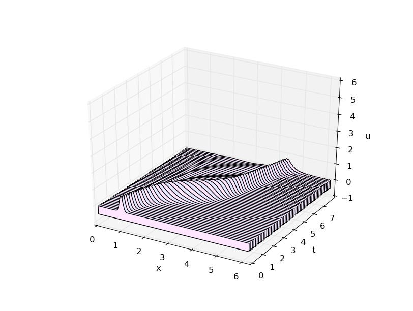
Numerical artifacts are very visible. (Bad!)
With spectral spatial derivative:
for j in range(1,m):
        # spatial derivative approximation at row j
        # spectral spatial derivative
        y = fft(w[j,:])
        kvals = hstack( [ range(n/2),  [0]  , range(-n/2+1,0) ] )
        yp = y*2*pi*1.j*kvals/L
        wx = real(ifft(yp))

        w[j+1,:] = w[j-1,:] - 2.*k*cgrid*wx
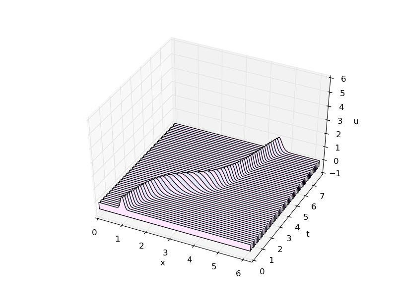
No artifacts! (Good!)
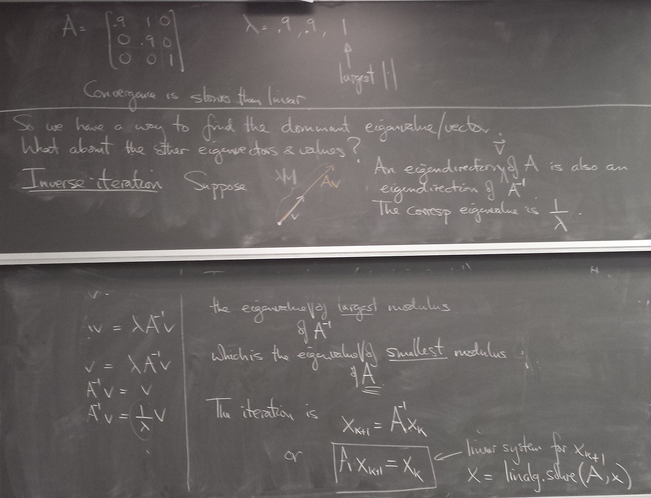
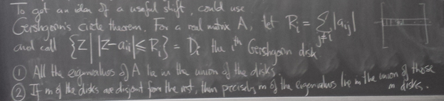
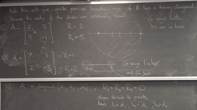
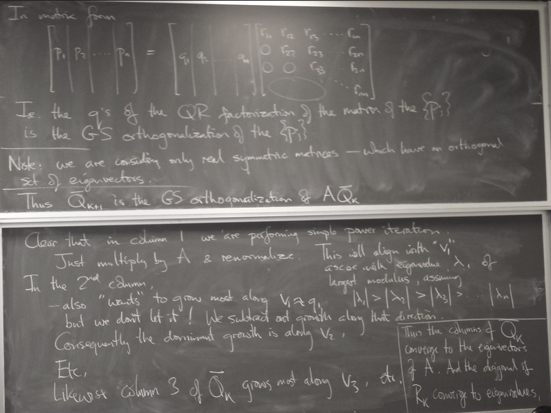
Computing eigenvalues and eigenvectors of matrices
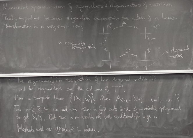
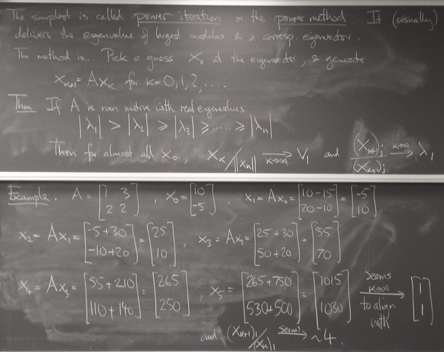
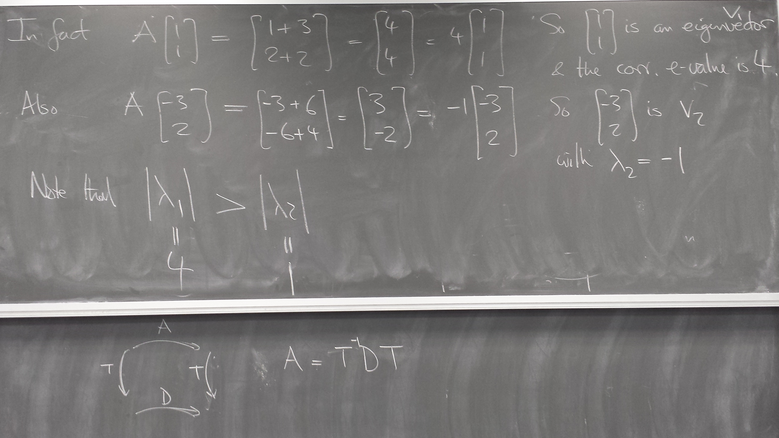
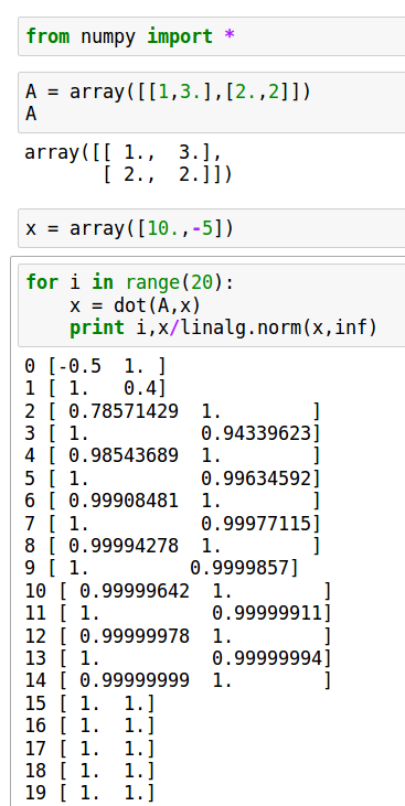
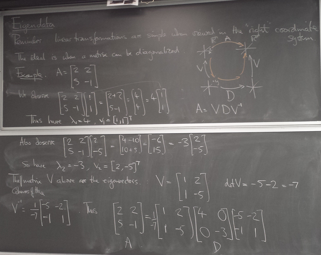
Power iteration
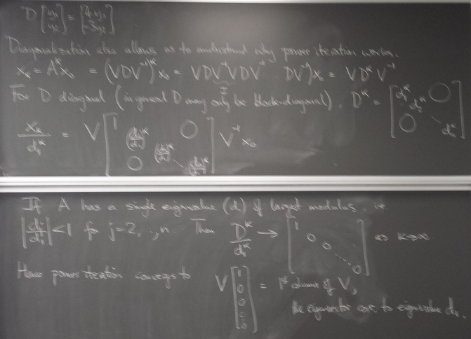
x = dot(a,x)
lam = norm(x,inf)
x /= lam
Illustrations:
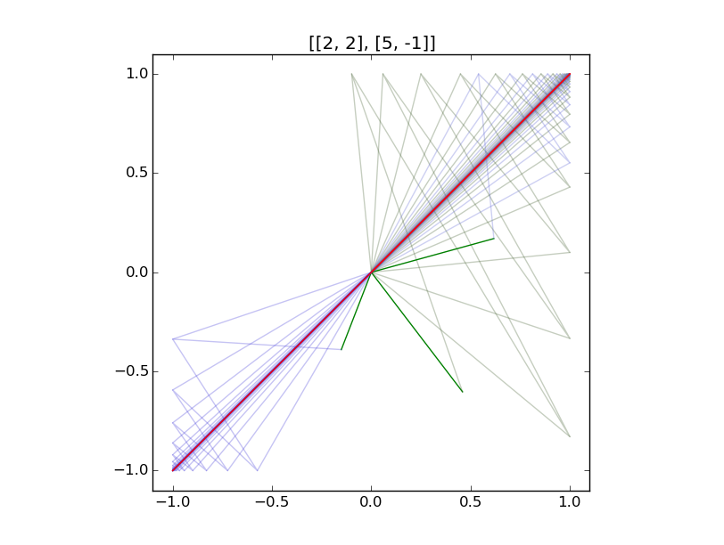
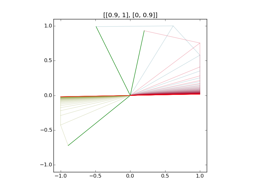

Examples of iteration of diagonalizable and non-diagonalizable transformations.
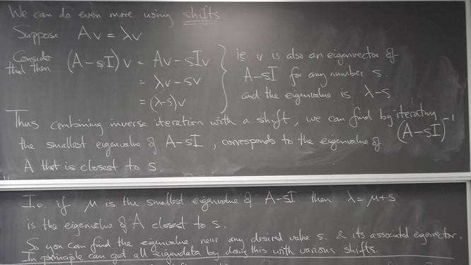
Inverse and shifted power iteration
Allows us to obtain the eigenvalue closest to any chosen number, and its eigenline.
QR algorithms
Construct an diagonalizing orthogonal similarity?
E.g. by Householder reflectors?
Impossible. But we can use this to obtain Hessenberg or tridiagonal form, which is useful from an efficiency standpoint.
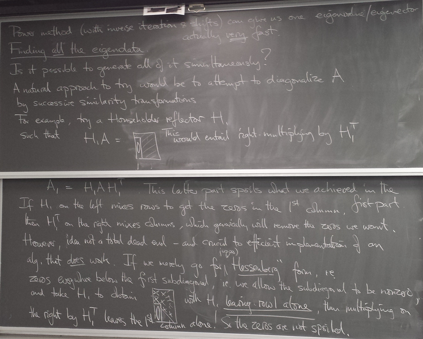
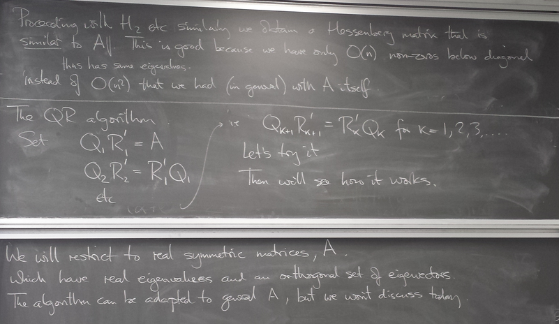
QR iteration on a real symmetric matrix A
Seems like a weird thing to do, but note that this is a sequence of similarity transformations.

let's try it and see what happens.
# implementation of pure QR iteration


from numpy import *

def cook_up_symmetric_matrix(n):
        a = random.randn(n,n)
        return a+a.T

a = cook_up_symmetric_matrix(3)

for i in range(100):  # do 100 iterations

        q,r = linalg.qr(a)
        a = dot(r,q)
        print('r')
        print(r.round(4))
        print('q')
        print(q.round(4))

# compare with eigenvalues given by linalg.eigvals()
print(linalg.eigvals(asave).round(4))
...
r
[[-4.9221  0.      0.    ]
 [ 0.      2.6202 -0.    ]
 [ 0.      0.      1.4494]]
q
[[-1. -0.  0.]
 [ 0. -1.  0.]
 [ 0.  0.  1.]]
r
[[-4.9221  0.     -0.    ]
 [ 0.      2.6202  0.    ]
 [ 0.      0.      1.4494]]
q
[[-1.  0. -0.]
 [-0. -1.  0.]
 [-0.  0.  1.]]
[ 4.9221  1.4494 -2.6202]
$
We see that if we form RQ, we have the eigenvalues on the diagonal.
If we don't want to rely on linalg.eigvals() to give us the "truth", we can build our own matrix with known eigenvalues that are not obvious by inspection. We simply take a diagonal matrix, whose eigenvalues are on the diagonal, and then apply a random similarity transformation (which preserves eigenvalues):
from numpy import *

def make_matrix_with_known_eigenvalues(lambdas):
        # start with diagonal and
        # apply a random similarity transformation
        n = len(lambdas)
        a = zeros((n,n))
        fill_diagonal(a,lambdas)
        r = random.randn(n,n)
        #print(a)
        return dot(r,dot(a,linalg.inv(r)))

a = make_matrix_with_known_eigenvalues([6.,-4.,1.234])
print 'A'
print a
asave = a.copy()

for i in range(100):  # do 100 iterations

        q,r = linalg.qr(a)
        a = dot(r,q)
        print('r')
        print(r.round(4))
        print('q')
        print(q.round(4))
$ python3 qrit2.py
A
[[  3.94899743   5.86042366  11.95073405]
 [  1.7048188    9.42478357   9.96527914]
 [ -2.57568658  -5.62617251 -10.139781  ]]
r
[[ -5.0135 -10.7114 -18.0112]
 [  0.      -6.3317  -4.4347]
 [  0.       0.      -0.933 ]]
q
[[-0.7877  0.4069  0.4626]
 [-0.34   -0.9132  0.2244]
 [ 0.5138  0.0195  0.8577]]
r
[[  1.7342  -7.4899  19.9292]
 [  0.      -5.5662   5.313 ]
 [  0.       0.       3.0681]]
q
[[-0.9583 -0.0384 -0.2831]
 [-0.0722 -0.9262  0.3702]
 [-0.2764  0.3752  0.8848]]

...

r
[[ -6.     -13.5473 -14.8379]
 [  0.       4.       8.2272]
 [  0.       0.       1.234 ]]
q
[[-1. -0.  0.]
 [ 0. -1.  0.]
 [-0.  0.  1.]]
r
[[ -6.     -13.5473  14.8379]
 [  0.       4.      -8.2272]
 [  0.       0.       1.234 ]]
q
[[-1.  0. -0.]
 [-0. -1.  0.]
 [ 0.  0.  1.]]
We see that after 100 iterations (and maybe many fewer), RQ has the prescribed eigenvalues on the diagonal.
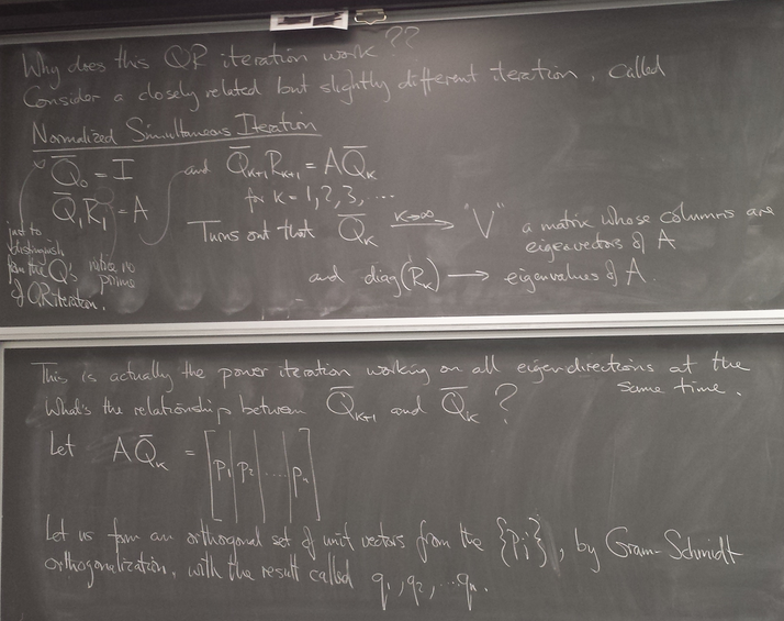
Why does it work?
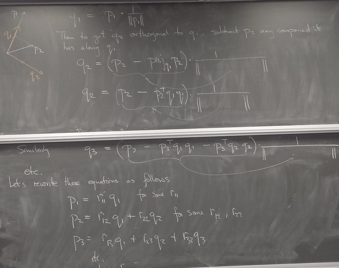
Normalized simultaneous iteration
for real symmetric matrices (which are diagonalizable by a real orthogonal matrix)
Gives us all the eigenvalues and eigenvectors at once!
Visualizations for project presentations
Every one of the project options provides opportunities for nice visualization of the results. Let's make sure every presentation contains good visualizations.
Thursday, April 28, 2016
Project presentations
Each student will present, and each student must as at least one question about another group's work.
Thursday, April 28, 2016
Project presentations: Shazam
Each student will present, and each student must as at least one question about another group's work.
May 5, 2016
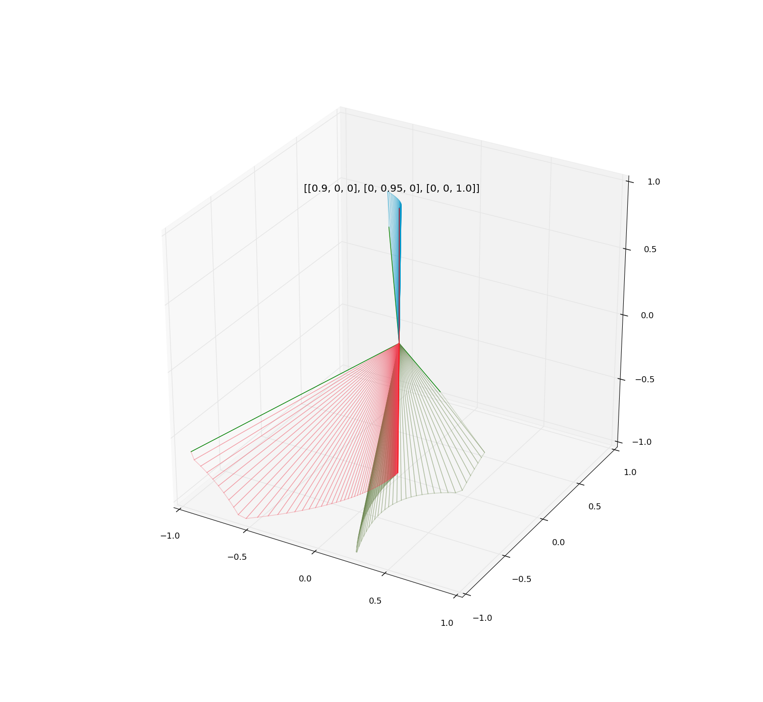
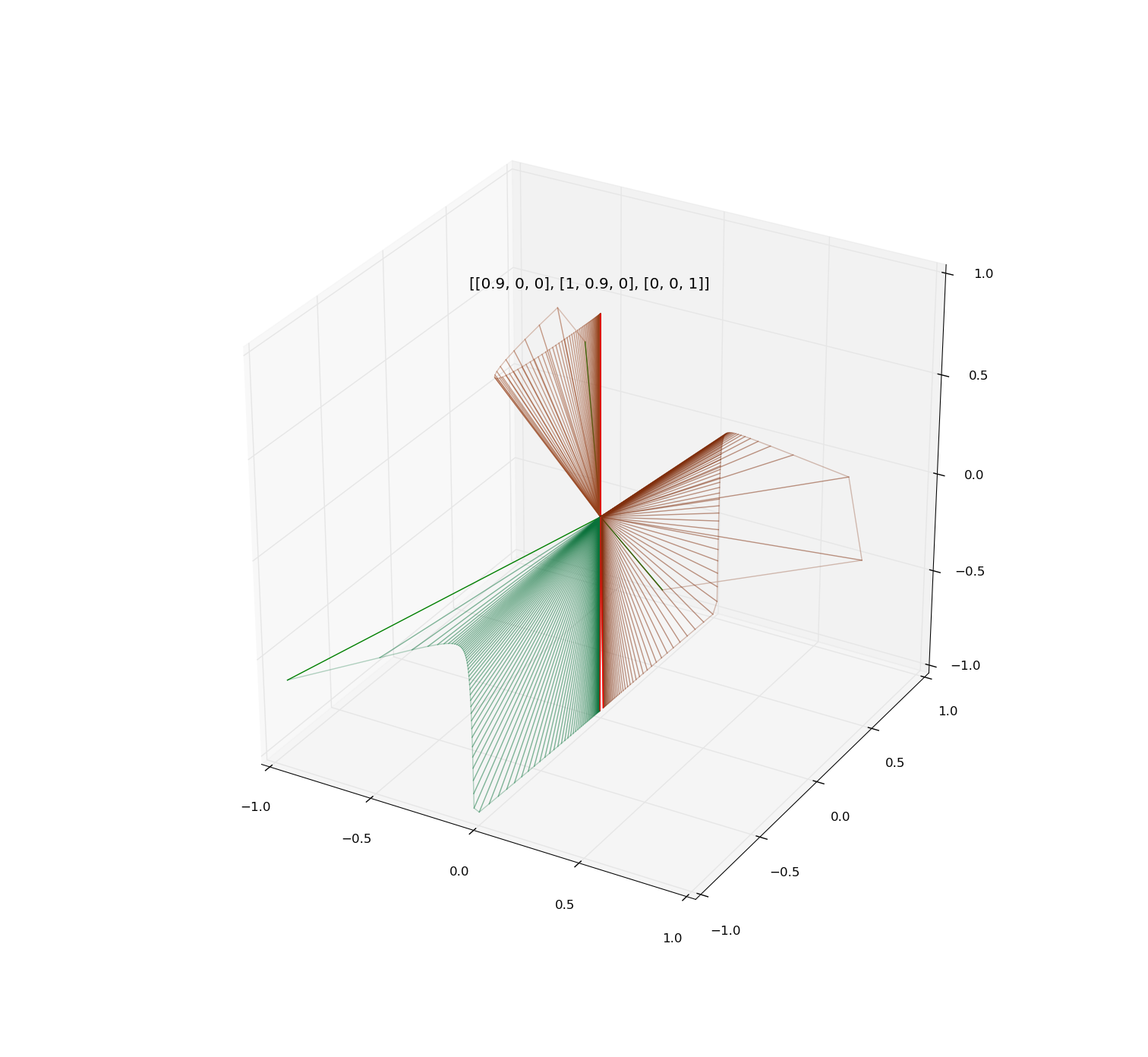
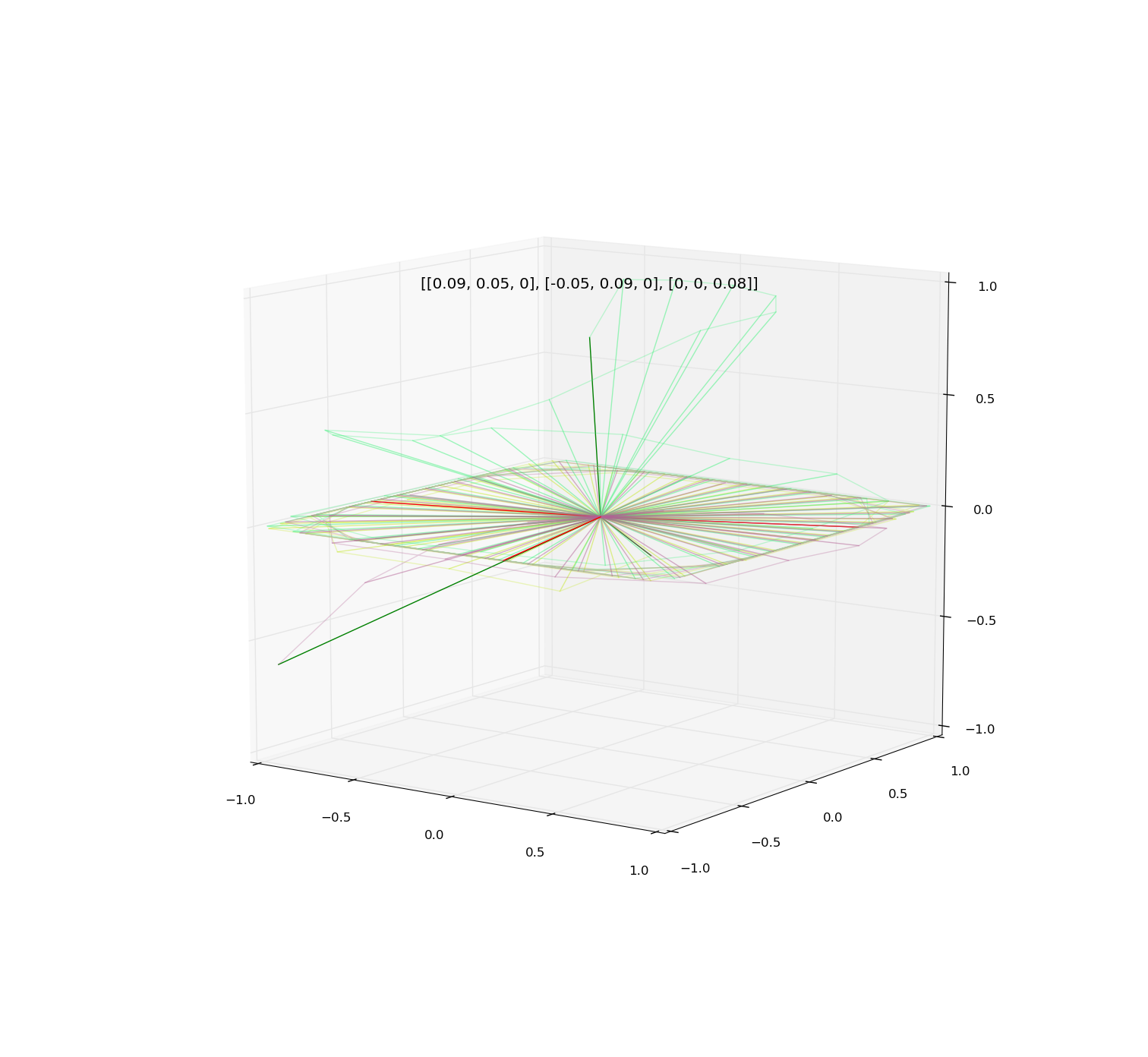
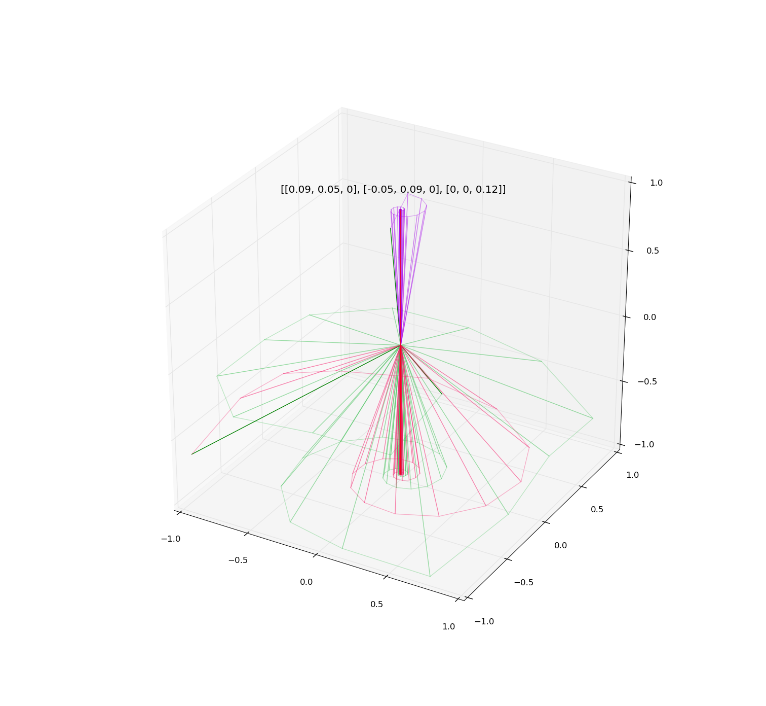
Singular Value Decomposition (SVD)
Image of unit sphere is hyperellipse
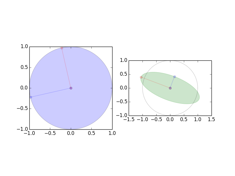
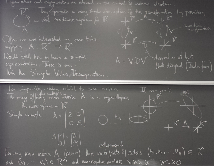
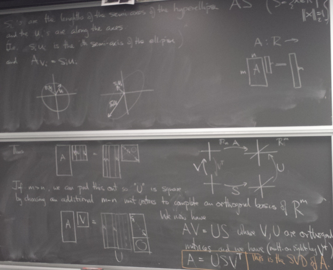
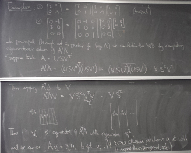
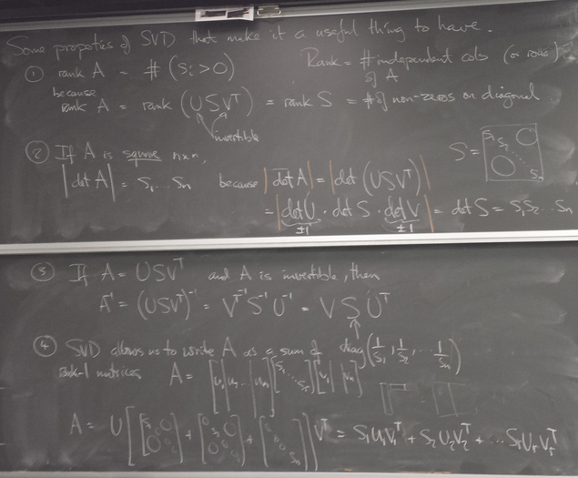
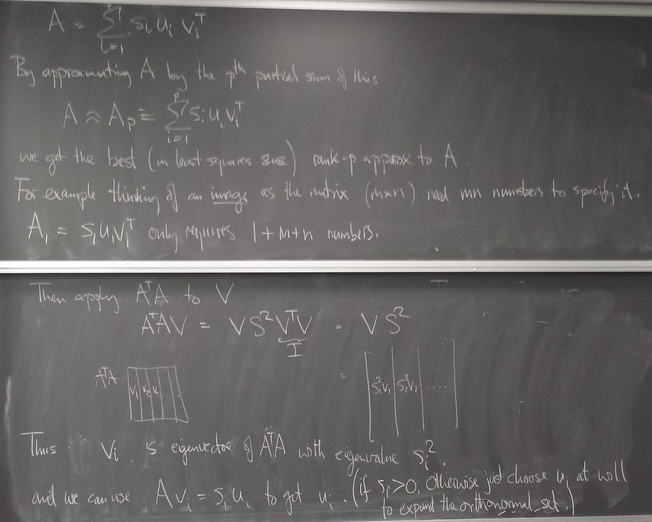
Image compression with SVD
Decomposition of matrix as a sum of rank-one matrices
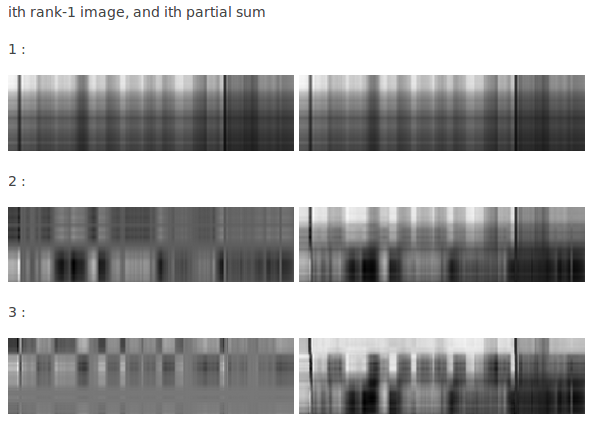
For more of the rank-1 images and their partial sums click here
Online course evaluations
Your thoughts and suggestions are valued.